Downloaded 193 times

![Snake -> Curves
Consider a closed planar curve C ( p) {x( p), y( p)}, p [0,1]
C(0.1)
S(p) is the arclength
C(0.2)
C(0.7)
C(0)
C(0.4)
C(0.95)
Cp =tangent
C(0.8)
Css
| Cp |
Css
N
N
1
C(0.9)
Cs
Cp
C
The geometric trace of the curve can be alternatively
represented implicitly as C {( x, y ) | ( x, y ) 0}
1
0
0
1](https://image.slidesharecdn.com/snakecurveslevelset-140129163014-phpapp01/85/Snakes-in-Images-Active-contour-tutorial-4-320.jpg)
![Properties of Level Sets
The level set curvature
Css =div
|
|
Proof. zero change along the level sets,
ss
So,
( x, y )
d
( x xs
ds
,
|
|
y
|
ys )
|
[
,T
d
ds
x
xx s
xy
ys ,
ss
,T
d
ds
x
xy s
yy
ys ],
|
0 , also
, N
|
Numerical Geometry of Images:
http://webcourse.cs.technion.ac.il/236861/Winter2012-2013/en/ho_Tutorials.html](https://image.slidesharecdn.com/snakecurveslevelset-140129163014-phpapp01/85/Snakes-in-Images-Active-contour-tutorial-6-320.jpg)
![Snake Model
1
arg min
C
Cp
0
2
C pp
tension
2
rigidity
2 g (C ) dp
external energy from the image
Energy
g (C )
|
[G (C ) * I (C )] |2
A snake that minimize E must satisfy the Euler equation
Cpp
Cpppp
g C
0
To find a solution
dC
dt
C pp
C pppp
g C
When C stabilizes and the term Ct vanishes, a solution is achieved.
Snakes: Active Contour Models, 1988](https://image.slidesharecdn.com/snakecurveslevelset-140129163014-phpapp01/85/Snakes-in-Images-Active-contour-tutorial-11-320.jpg)
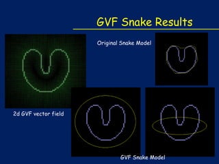
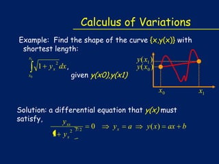
![GVF Snakes
Replace the external force with gradient vector flow (GVF) force v.
dC
dt
C pp
C pppp
g C
V(x,y) = [u(x,y),v(x,y)]
Why?
f generally have large magnitudes only in the vicinity of the edges, the
capture range would be small.
It’s nearly zero in homogeneous regions.
V(x,y) = [u(x,y), v(x,y)] is defined as the vector field that minimizes
the energy functional:
http://www.iacl.ece.jhu.edu/static/gvf/](https://image.slidesharecdn.com/snakecurveslevelset-140129163014-phpapp01/85/Snakes-in-Images-Active-contour-tutorial-13-320.jpg)


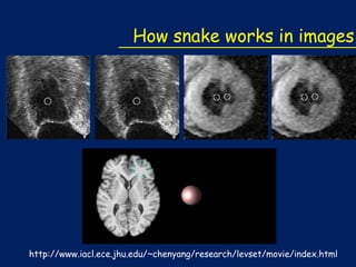
The document describes how snakes, or active contours, can be used to model shapes in images. It discusses how snakes work by defining an energy function along a curve and minimizing that energy to find the optimal curve. The energy includes an internal term based on curvature and an external term from image features. Level sets are used to propagate the curves towards the minimum energy configuration using gradient descent. Key steps include modeling the shape as a curve, defining the energy function, deriving the curve to minimize energy via calculus of variations, and propagating the curves using level sets.