The document provides information about computer graphics concepts including:
1. Summarizing questions and answers about 3D triangles, rotation matrices, vector operations, splines, and computer graphics techniques like environment mapping and anti-aliasing.
2. Explaining modifications made to the active edge list algorithm to enable scan conversion of different triangle types like smoothly shaded, textured, and environment mapped triangles.
3. Deriving the 4x4 projection matrix that maps a 3D object point to its shadow point on a plane, to create planar shadows.
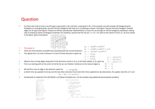
Build Your Own 3D Scanner: Surface ReconstructionDouglas Lanman
Build Your Own 3D Scanner:
Surface Reconstruction
http://mesh.brown.edu/byo3d/
SIGGRAPH 2009 Courses
Douglas Lanman and Gabriel Taubin
This course provides a beginner with the necessary mathematics, software, and practical details to leverage projector-camera systems in their own 3D scanning projects. An example-driven approach is used throughout; each new concept is illustrated using a practical scanner implemented with off-the-shelf parts. The course concludes by detailing how these new approaches are used in rapid prototyping, entertainment, cultural heritage, and web-based applications.
In Computer Graphics, Hidden surface determination also known as Visible Surface determination or hidden surface removal is the process used to determine which surfaces
of a particular object are not visible from a particular angle or particular viewpoint. In this scribe we will describe the object-space method and image space method. We
will also discuss Algorithm based on Z-buffer method, A-buffer method, and Scan-Line Method.
I am Danny G . I am an Electrical Engineering Assignment Expert at matlabassignmentexperts.com. I hold a Ph.D. Matlab, Schiller International University, USA. I have been helping students with their homework for the past 9 years. I solve assignments related to Electrical Engineering.
Visit matlabassignmentexperts.com or email info@matlabassignmentexperts.com.
You can also call on +1 678 648 4277 for any assistance with Electrical Engineering Assignments.
Dear students get fully solved assignments
Send your semester & Specialization name to our mail id :
help.mbaassignments@gmail.com
or
call us at : 08263069601
Image segmentation is a computer vision task that involves dividing an image into multiple segments or regions, where each segment corresponds to a distinct object, region, or feature within the image. The goal of image segmentation is to simplify and analyze an image by partitioning it into meaningful and semantically relevant parts. This is a crucial step in various applications, including object recognition, medical imaging, autonomous driving, and more.
Key points about image segmentation:
Semantic Segmentation: This type of segmentation assigns each pixel in an image to a specific class, essentially labeling each pixel with the object or region it belongs to. It's commonly used for object detection and scene understanding.
Instance Segmentation: Here, individual instances of objects are separated and labeled separately. This is especially useful when multiple objects of the same class are present in the image.
Boundary Detection: Some segmentation methods focus on identifying the boundaries that separate different objects or regions in an image.
Methods: Image segmentation can be achieved through various techniques, including traditional methods like thresholding, clustering, and region growing, as well as more advanced techniques involving deep learning, such as using convolutional neural networks (CNNs) and fully convolutional networks (FCNs).
Challenges: Image segmentation can be challenging due to variations in lighting, color, texture, and object shape. Overlapping objects and unclear boundaries further complicate the task.
Applications: Image segmentation is used in diverse fields. For example, in medical imaging, it helps identify organs or abnormalities. In autonomous vehicles, it aids in identifying pedestrians, other vehicles, and obstacles.
Evaluation: Measuring the accuracy of segmentation methods can be complex. Metrics like Intersection over Union (IoU) and Dice coefficient are often used to compare segmented results to ground truth.
Data Annotation: Creating ground truth annotations for segmentation can be labor-intensive, as each pixel must be labeled. This has led to the development of datasets and tools to facilitate annotation.
Semantic Segmentation Networks: Deep learning architectures like U-Net, Mask R-CNN, and Deeplab have significantly improved the accuracy of image segmentation by effectively learning complex patterns and features.
Image segmentation plays a fundamental role in understanding and processing images, enabling computers to "see" and interpret visual information in ways that mimic human perception.
Image segmentation is a computer vision task that involves dividing an image into meaningful and distinct segments or regions. The goal is to partition an image into segments that represent different objects or areas of interest within the image. Image segmentation plays a crucial role in various applications, such as object detection, medical imaging, autonomous vehicles, and more.
Dear students get fully solved assignments
Send your semester & Specialization name to our mail id :
“ help.mbaassignments@gmail.com ”
or
Call us at : 08263069601
Graph Analytics - From the Whiteboard to Your Toolbox - Sam LermaPyData
However, the the graph theory jargon can make graph analytics seem more intimidating for self-study than is necessary. In this talk, the audience will be exposed to some of the basic concepts of graph theory (no prerequisite math knowledge needed!) and a few of the Python tools available for graph analysis.
This slide is special for master students (MIBS & MIFB) in UUM. Also useful for readers who are interested in the topic of contemporary Islamic banking.
Executive Directors Chat Leveraging AI for Diversity, Equity, and InclusionTechSoup
Let’s explore the intersection of technology and equity in the final session of our DEI series. Discover how AI tools, like ChatGPT, can be used to support and enhance your nonprofit's DEI initiatives. Participants will gain insights into practical AI applications and get tips for leveraging technology to advance their DEI goals.
How to Build a Module in Odoo 17 Using the Scaffold MethodCeline George
Odoo provides an option for creating a module by using a single line command. By using this command the user can make a whole structure of a module. It is very easy for a beginner to make a module. There is no need to make each file manually. This slide will show how to create a module using the scaffold method.
Acetabularia Information For Class 9 .docxvaibhavrinwa19
Acetabularia acetabulum is a single-celled green alga that in its vegetative state is morphologically differentiated into a basal rhizoid and an axially elongated stalk, which bears whorls of branching hairs. The single diploid nucleus resides in the rhizoid.
June 3, 2024 Anti-Semitism Letter Sent to MIT President Kornbluth and MIT Cor...Levi Shapiro
Letter from the Congress of the United States regarding Anti-Semitism sent June 3rd to MIT President Sally Kornbluth, MIT Corp Chair, Mark Gorenberg
Dear Dr. Kornbluth and Mr. Gorenberg,
The US House of Representatives is deeply concerned by ongoing and pervasive acts of antisemitic
harassment and intimidation at the Massachusetts Institute of Technology (MIT). Failing to act decisively to ensure a safe learning environment for all students would be a grave dereliction of your responsibilities as President of MIT and Chair of the MIT Corporation.
This Congress will not stand idly by and allow an environment hostile to Jewish students to persist. The House believes that your institution is in violation of Title VI of the Civil Rights Act, and the inability or
unwillingness to rectify this violation through action requires accountability.
Postsecondary education is a unique opportunity for students to learn and have their ideas and beliefs challenged. However, universities receiving hundreds of millions of federal funds annually have denied
students that opportunity and have been hijacked to become venues for the promotion of terrorism, antisemitic harassment and intimidation, unlawful encampments, and in some cases, assaults and riots.
The House of Representatives will not countenance the use of federal funds to indoctrinate students into hateful, antisemitic, anti-American supporters of terrorism. Investigations into campus antisemitism by the Committee on Education and the Workforce and the Committee on Ways and Means have been expanded into a Congress-wide probe across all relevant jurisdictions to address this national crisis. The undersigned Committees will conduct oversight into the use of federal funds at MIT and its learning environment under authorities granted to each Committee.
• The Committee on Education and the Workforce has been investigating your institution since December 7, 2023. The Committee has broad jurisdiction over postsecondary education, including its compliance with Title VI of the Civil Rights Act, campus safety concerns over disruptions to the learning environment, and the awarding of federal student aid under the Higher Education Act.
• The Committee on Oversight and Accountability is investigating the sources of funding and other support flowing to groups espousing pro-Hamas propaganda and engaged in antisemitic harassment and intimidation of students. The Committee on Oversight and Accountability is the principal oversight committee of the US House of Representatives and has broad authority to investigate “any matter” at “any time” under House Rule X.
• The Committee on Ways and Means has been investigating several universities since November 15, 2023, when the Committee held a hearing entitled From Ivory Towers to Dark Corners: Investigating the Nexus Between Antisemitism, Tax-Exempt Universities, and Terror Financing. The Committee followed the hearing with letters to those institutions on January 10, 202
2. Question
• 1.Consider a 3D triangle with vertices (0,0,0), (5,0,10), (0,20,0). What is the z value of the point in the triangle with x=3, y=1?
• The question is, what linear combo of the 3 vertices matches the x and y components of (3,1,z)? (3,1) = .6 (5,0) + .05 (0,20). So the answer is
z= .6x10+.5x0 = 6.
• 2.Why can the following not possibly be a 3D Cartesian rotation matrix?
• column 2 doesn't have length =1. Various other reasons are also ok.
• 3.If a=(4,3,5) then write (a⋅p)a as a matrix M, depending only on a, times p.
• 4.What is the 4x4 homogeneous matrix for a 3D rotation by 90 degrees about the X axis, followed by this translation: x'=x-1, y'=y+1, z'=z+2.
• 5.Write the vector formula for the 3D rotation by 60 degrees about the Y axis.
• 6.Write the quaternion for the 3D rotation by 60 degrees about the Y axis.
• 7.What is one problem with interpolating a spline through the control points instead of approximating a spline near the points?
• The curve will swing outside the convex hull of the control points, by an amount that is not intuitive. If the control points are almost collinear, the
curve might not be. IOW, it's harder to predict the curve from the control points.
• 8.What advantage do cubic splines have over quadratic splines?
• You can match the curve sections with their first two derivatives and the joint, making the joint generally invisible.
• 9.What technique computes the surroundings visible as a reflected image in a shiny object?
• environment mapping
• 10.When projected objects are less than one pixel large, there is a lot of fictitious high frequency clutter in the image. Name the technique used to fix
this.
• anti-aliasing
• 11.In the graphics pipeline, does the rasterizer send its output to the vertex or fragment shader? (Pick one, or pick both.)
• fragment shader.
• 12.In the graphics pipeline, when a triangle is processed, the (x,y,z) coordinates of the vertices are interpolated across the whole triangle to give the
coordinates of each fragment. Name two other things that may commonly be specified at the vertices and then interpolated across the triangle to
give a value for each fragment.
• colors, normals.
3. Question continue
• 13.Where in the graphics pipeline does texture mapping take place?
• fragment shader.
• 14.When clipping in 3D, how many independent clippers are required in the pipeline?
• 6.
• 15.Do a view normalization of this square A(3,3), B(3,4), C(4,4), D(4,3) that is being viewed from (0,0) and projected into the plane x=1. The
transformed square, when seen with a parallel projection from x= -infinity should look the same as the original square when seen in perspective from
(0,0). That is, write the transformed coordinates for ABCD. Also, draw a figure showing the projection.
• 16.Are vertices assembled into objects in the vertex shader, in the fragment shader, or in the rasterizer?
• rasterizer.
• 17.Draw an example where clipping a polygon causes it to split into two pieces (connected by edges running along the edge of the clip window).
• 18.Draw 1/8 of a circle of radius R=12 using the Bresenham method. Show your work.
• 19.Following the principle that less is more, the OpenGL designers decided not to include some functionality that a program that processes images
would probably need. Name it.
• Reading and writing image files.
• 20.When compositing several images, the limited precision of the color (frame) buffers may hurt the image quality. Therefore, OpenGL also has
another buffer to composit into. Name it.
• Accumulation buffer.
• 21.Is the following code a vertex shader or a fragment shader? void main(void) { gl_FragColor = gl_FrontColor;}
• Fragment shader.
• 22.Do you set a texture coordinate thus glTexCoord2f(s0, t0); before or after the vertex it applies to?
• Before.
• 23.Can the standard OpenGL pipeline easily handle light scattering from object to object? Why (not)?
• No, because it processes vertices independently, often in separate graphics cores, and they cannot easily interact with each other.
• // diffuse.fs: per-pixel diffuse lighting varying vec3 N, L;
• void main(void)
• { // output the diffuse color
• float intensity = max(0.0, dot(normalize(N), normalize(L)));
• gl_FragColor = gl_Color;
• gl_FragColor.rgb *= intensity; }
• 24.Where do the variables N and L get their values from?
• Computed by the rasterizer (from per-vertex values supplied by the vertex shader).
• 25.What uses the value of the variable gl_FragColor?
• It becomes the color of the pixel, if this fragment passes other tests like the depth buffer.
4. Question
• You have learned about parametric and geometric continuity. For each 2D curve, answer the continuity query as correctly as possible, and provide a
brief explanation:
• (a) Is a circle C0 continuous?
• The answer is:
• Parametric “C” continuity refers to the continuity of the parameterization used. However, since no parameterization has been specified, the question
is ambiguous—circle parameterizations may or may not be C0.
• (b) Is a circle G0 continuous?
• The answer is:
• Geometric “G” continuity refers to the continuity of the geometric shape. Yes the circle is G0 continuous because the curve is connected (unbroken)
everywhere.
• (c) Is a circle C∞ continuous?
• The answer is:
• Again it is unclear, since no parameterization has been specified. Circle parameterizations may or may not be C0.
• (d) Is a circle G ∞ continuous?
• The answer is:
• Yes, because the circle is infinitely smooth. It can also be parameterized by (x(t); y(t)) = (sin(t); cos(t)) which is infinitely differentiable.
• (e) Is a square C0 continuous?
• The answer is:
• Unclear, since no parameterization has been specified. Parameterizations of the square may or may not be C0.
• (f) Is a square G0 continuous?
• The answer is:
• Yes, because the curve is continuous/unbroken everywhere.
• (g) Is a square C1 continuous?
• The answer is:
• Unclear, since no parameterization has been specified. Parameterizations may or may not be C1, even though there are corners.
• (h) Is a square G1 continuous?
• The answer is:
• No, because tangents to the geometric curve have direction discontinuities at the corners.
5. Question
• This question explores how the active edge list algorithm has evolved.
• a) Describe how the active edge list algorithm is used to scan convert a constant-color triangle.
• The answer is:
• Proceeding in scan line order from the top-to-bottom (or, equivalently, bottom-to-top), the active edge list algorithm maintains (possibly in a list) the
leftmost and rightmost edge of the triangle, indicating the pixels that fall within the triangle’s boundary and which should be filled in the scan line.
• b) What modifications are made to it to enable it to scan convert a smoothly-shaded triangle?
• The answer is:
• At each scan line, the algorithm linearly interpolates the vertex colors of the vertices bounding each edge to get two “edge colors”. Then, as it
generates pixels, the algorithm linearly interpolates the edge colors for each pixel.
• c) What modifications are made to it to enable it to scan convert a textured triangle?
• The answer is:
• Each vertex maps to a coordinate in texture space. As in (b), these coordinates are interpolated to get edge texture coordinates and, as the algorithm
generates pixels, those texture coordinates are again interpolated to get the texel values that each pixel is set to.
• d) What modifications are made to it to enable it to scan convert an environmentmapped triangle?
• The answer is:
• Vertex normals, not coordinates, map into positions in the environment map. Thereafter, the same considerations as in (c) apply.
• e) What modifications are made to it to enable it to scan convert a triangle rendered with Phong shading?
• The answer is:
• As in (b), except that it is the normals themselves that are interpolated, first at the edges and then at each pixel. Then the lighting model itself
(OpenGL or whatever) computes the color at each pixel.
6. Question
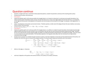
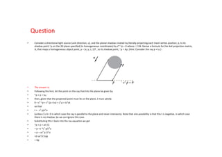
• Consider the animation of a spherical particle of radius r moving with constant velocity v towards a wall at the z = 0 plane. Given an initial position p0
at t = 0 that is farther from the wall than r, the position of the particle center at any later time t prior to the collision is given by: p(t) = p0 + vt
• (a) At what time will the particle contact the wall?
• The answer is: tb =(r − pz)/ vz
• (b) Let tb (“time of bounce”) be the solution to Part 3a. Since this is an an animation, you only render frames at discrete multiples of the frame time t
(i.e., t = 0,t, 2t, 3t, ...). If tb is not a multiple of t – and in general, it isn’t – the animated particle can penetrate the wall from the time step before tb
to the one after it.
• Give (pseudo)code for computing p[] in this:
• // given:
• int n; // the number of frames to render (a positive int)
• float dt; // time step
• float v[3]; // the initial velocity of the particle
• float p0[3]; // the initial position of the particle
• float r; // the radius of the particle
• // derived:
• float tb = // assume you have the answer to (3a)
• float p[3];
• for (int i = 0; i < n; i++) { // i is the frame number
• // compute p[] <-- your code goes here
• drawParticle(p, r);
• }
• Allow for the possibility of collision. Assume an elastic collision, so that the effect of the “bounce” is to negate the z component of v (i.e. v[2]) but
leave the x and y components alone.
• The answer is:
• t = i * dt;
• p[0] = p0[0] + t * v[0]
• p[1] = p0[1] + t * v[1]
• if (t < tb)
• p[2] = p0[2] + t * v[2]
• else
• p[2] = r - v{2] * (t - tb)
7. Question
• Consider a directional light source (unit direction, u), and the planar shadow created by literally projecting each mesh vertex position, p, to its
shadow point ~p on the 3D plane specified (in homogeneous coordinates) by cT ~p = 0 where c 2 R4. Derive a formula for the 4x4 projection matrix,
A, that maps a homogeneous object point, p = (x; y; z; 1)T , to its shadow point, ~p = Ap. (Hint: Consider the ray p + tu.)
• The answer is:
• Following the hint, let the point on the ray that hits the plane be given by
• ~p = p + tu;
• then, given that the projected point must lie on the plane, t must satisfy
• 0 = cT ~p = cT (p + tu) = cT p + tcTut
• so that
• t = - cT p/cTu
• (unless cTu 6= 0 in which case the ray is parallel to the plane and never intersects). Note that one possibility is that this t is negative, in which case
there is no shadow, be we can ignore this case.
• Substituting this t back into the ray equation we get
• ~p = p + ut (1)
• = p –u *cT p/cTu
• = p – ucT p /cTu
• =(I-ucT/cTu)p
• = Ap
8. Question
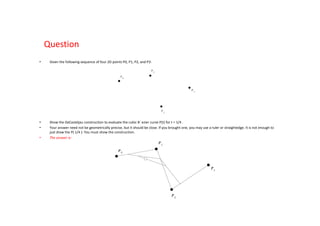
• Consider the cubic spline segment, p(t) = a t3 + b t2 + c t + d; on the unit interval t 2 [0; 1]. Recall that Hermite splines use p and p0 controls at each
end point, i.e., p0 = p(0), p0 0 = p0(0), p1 = p(1), p0 1 = p0(1). In this question you will derive a spline which instead uses the following controls: at t =
0, use position (p0), velocity (p0 0) and acceleration (p00 0); at t = 1, use position (p1).
• (a) What is this spline’s 4x4 geometry matrix G such that
• The answer is:
• Taking derivatives of p(t) we have
• so that
• It follows that
• Therefore the curve and geometry matrix are given by
• (b) Given a cubic spline contructed from these segments, is the resulting curve (i) C0 continuous? (ii) C1 continuous? (iii) G0 continuous? (iv) G1
continuous? Briefly explain your reasoning in each case.
• The answer is:
• The question asks you to consider continuity at the endpoints of a spline segment. You can assume that we have a spline that has uniformly spaced
knots, with each knot specified by triples of values (p0, p0 0, p00 0) at t = 0, then (p1, p0 1, p00 1) at t = 1, then (p2, p0 2, p00 2) at t = 2, etc. Assume
that we have two spline segments, p(t) for t 2 [0; 1] and a separate q(t) for t 2 [1; 2] (which could be mapped to our [0,1] derivation by a translation,
= t 1), and that we will consider what happens at t = 1. Since the cubic spline constructed by joining these segments is geometrically connected at t =
1 (it must share the same endpoint p1) it must have G0 geometric continuity. Furthermore, since the coordinate functions are cubic polynomials
(which are continuous to all orders), then the curve must also have the same limits at t = 1, i.e., limt! p(t) = limt!1+ q(t) = p1, and therefore it must
have C0 parametric continuity. However, unlike the Hermite cubic spline, there is no reason that the curve’s tangents should be equal at the
endpoints; the values of p0(1) and q0(1) depend on different control parameters, (p0, p0 0, p00 0, p1) and (p1, p0 1, p00 1, p2), respectively, and
therefore we won’t have C1 parametric continuity. Furthermore, since the endpoint tangents needn’t even point in the same direction, we can’t
have G1 geometric continuity either.
9. Question
• Given the following sequence of four 2D points P0, P1, P2, and P3:
• Show the DeCasteljau construction to evaluate the cubic B´ezier curve P(t) for t = 1/4 .
• Your answer need not be geometrically precise, but it should be close. If you brought one, you may use a ruler or straightedge. It is not enough to
just draw the P( 1/4 ): You must show the construction.
• The answer is:
10. Question
• Transforms in OpenGL are represented by a 4 x 4 matrix whose elements are given by mi:
•
• OpenGL functions that act on the matrix on the top of the currently-selected matrix stack (depending on the matrix mode – GL MODELVIEW, GL
PROJECTION, or GL TEXTURE) effectively multiply it in place by another matrix we’ll call an “effective matrix” E, which is an identity matrix with
certain elements modified according to the function arguments.
• For example, the effective matrix for glTranslate[df](x, y, z) is an identity matrix with m12, m13, and m14 modified by the function’s arguments:
• a) Fill in the following table to indicate which elements of E (starting out as an identity matrix in each case) would be affected by the arguments
of the given OpenGL function(s). Do not give the formula for each element, just a list of which elements get modified. This has already been
done for glTranslate[df]() as illustration.
• Do not assume anything about the values of the arguments passed. (i. e., It doesn’t matter that glTranslate[df](0.0, 0.0, 0.0) doesn’t really
change the values of the matrix.)
• The answer is:
• b) Consider a modelview matrix represented as in (a) as a change of coordinates from a “model” coordinate system to a “view” coordinate
system. In terms of the elements mi, what are the components of ˆz′, the direc on of the model’s ˆz unit vector in the view coordinate system?
(Remember that ˆz′ is of unit length.)
• The answer is:
11. Question
• Spheres are very popular objects to render in OpenGL. (Teapots are a close second!) A researcher using OpenGL for the first time specifies five
spheres arranged in an “X”, a light source, and a viewpoint fairly close to the spheres. The resulting image looks like this:
• The researcher is somewhat surprised! The sphere in the middle looks okay, but the surrounding spheres appear ellipsoidal! If you hold a ball in
space, even if you don’t look directly at it, it always appears spherical. After thinking about it for a minute, the researcher decides that the software is
not broken, but is (as usual with software) doing exactly what it was asked to do. Can you explain why the outer spheres appear ellipsoidal? (Hint:
You may want to make a sketch of the viewing geometry to clarify your point, but be sure to explain your point verbally in any case.)
• The answer is:
• The perspective projection of a sphere onto a viewing plane is ellipsoidal when the sphere is viewed off axis. The ellipticity is further enhanced when
the center of projection is close to the plane and the scene is viewed at an extremely wide angle. (Move your eyeball really close to the page to
simulate this: The ellipsoids will look spherical.)
12. Question
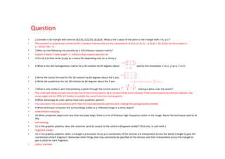
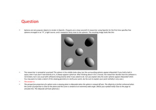
• Uniform subdivisions are commonly used for ray tracing, wherein a ray is intersected with cell boundaries to “walk” through the subdivision’s cells. In
this problem, you will generate pseudocode to walk through a uniform triangular subdivision (see figure). It can be viewed as the union of three 1D
uniform subdivisions (color-coded for convenience), each associated with a normalized direction vector (n0, n1 or n2). Each 1D cell is of width, h.
Denote each triangular cell by a 3-index label [i0, i1, i2] (RGB color coded) based on the cell’s location in each of the 1D subdivisions. Assume that our
ray r(t) originates from the origin, 0, so that r(t) = 0 + tu, t > 0. Assume that the origin lies at the centroid of the triangular cell indexed by [0, 0, 0].
• Write pseudocode to efficiently generate the sequence of traversed cells when given the ray direction, u and these particular cell direction vectors
(assume normalized). For example, given the u vector shown in the figure, your code would output the infinite sequence:
• [0, 0, 0], [1, 0, 0], [1, 1, 0], [1, 1, 1], [1, 2, 1], …Output a traversed cell with the function “output [i0, i1, i2].”
• The answer is:
• This is basically another ray-plane intersection problem. The rate at which the ray r(t) travels along the unit cell directions ni is given by the
component of r0 = u along each ni direction. In otherwords, the rate of position change in direction i is given by uTni, and since each direction must
travel h far between line crossings, the change in t between crossings for direction i is given by
• which may be negative. The remaining question is how far each direction must travel before reaching the first crossing, and this is related to the
position of the origin at the centroid of the [0,0,0] triangle. A simple geometric fact (that you can easily show) is that for an equilateral triangle placed
flat against the ground, of height h, the centroid occurs at height h=3. Therefore for directions n0 and n2, if their ti > 0 they must travel a distance
h=3 to their first crossing, but for ti < 0 its a distance of 2h=3. Unfortunately n1 is somewhat backwards: for positive t1 it must travel 2h=3, but for
negative t1 it must travel h=3. These spatial distances can be converted to t distances as with ti in. The algorithm then proceeds as follows. For each
direction i, we computeti, and initialize a variable tnext i for the next crossing time. The cell indices are set to [0,0,0]. At each step, we find the k
associated with the smallest tnext k , increment/decrement ik by 1 (depending on the sign of tk), increase tnext k by jtkj, and output [i0, i1, i2].
Pseudocode to do this is given below.
• For speed we could precompute/cache the jtkj and sign(tk) constants used in the forever loop.
13. Question
• In this question you will extend Bresenham’s midpoint algorithm for line rasterization to build a DDA-based rasterizer for a quadratic B´ezier curve.
For simplicity you may assume that the curve is parameterized in the form
• Where
• are the quadratic Bernstein polynomials. You may even assume that the slope of the curve satisfies 0< y’(x)< 1.
• (a) First, derive the equations needed to use forward differencing to evaluate the B´ezier curve at unit x = 1 spacings without unnecessary
multiplication. (Hint: First convert y(x) to monomial form.)
• The answer is:
• First convert to monomial form as suggested:
• Forward differences are easier than for the cubic case done in class. The first difference is
• and the second difference is
• with all higher differences zero. In summary, we must update y each increment by just adding 2a to it,
• and we update y by adding y(x),
• (b) Second, provide pseudocode for a simple DDA rasterizer from x = x0 to x = x1. You need not consider shading, attribute interpolation, or
antialiasing—you only need to “turn on” pixels using appropriate calls to output(x,y).
• The answer is:
• The pseudocode is identical to the original midpoint code, except with the line-based DDA update for y replaced by the forward-difference update
for the B´ezier curve. Recall that for line rasterization, each time we incremented x or y by 1, we updated the residual variable, d = mx + b - y, by m
or 1, respectively:
• The appropriate d variable for our problem is
• Incrementing y will still decrement d by 1, however now
• incrementing x will use the forward difference update, y(x).
• The pseudocode is as follows:
14. Question
• You have seen how to trace a ray through a square grid in 2D, and even a voxel grid in 3D. In this question you will consider 2D hexagonal grids.
Analogous to rectangular grids, assume that the hexagonal cells have an (i; j) indexing as shown in the figure. Assume that each hexagon’s parallel
edges are 2h apart (see figure). Propose an efficient pseudocode implementation to trace the ray through an infinite hexagonal subdivision, making
calls to output(i,j) indices of hexagons traversed. For simplicity, assume that the ray r(t) = e + tv, t >0, starts at the center of cell (i; j) = (0; 0) as shown
in the figure. Ignore boundaries.
• The answer is:
• There are three families of parallel lines associated with the normal directions
• The signed time t to travel a distance h in each of these directions is given by
• Observe that crossing edges along each of the directions results in an (i; j) cell index update, (i; j)+, given by
• From our starting point at the center of cell (0; 0), we can initialize t-distances to the nearest edges as
• We will first cross an edge in the direction i given by
• at which time we updateti to be 2jij, but the two other directions must have their times updated too. By observation, the update rules (for j 6= i) are
• Pseudocode to implement this HEX-WALK is as follows (multiplies by 2 can be avoided using additional precomputed variables):
15. Question
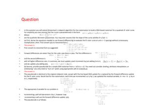
• Recall that Phong Shading interpolates vertex normals across a triangle for smooth shading on low-resolution meshes, i.e., the unnormalized surface
normal at barycentric coordinate (u; v;w) (where w = 1 - u - v) is approximated by barycentrically interpolated vertex normals,
• where the unit vertex normals are ni, nj and nk. Of course, since each triangle is still planar,
• the piecewise planar shape is still apparent at silhouettes.
• Recently, Boubekeur and Alexa [SIGGRAPH Asia 2008] introduced Phong Tesselation as a simple way to use vertex normals to deform a triangle mesh
to have smoother silhouettes (see Figures 1 and 2). In the following, you will derive their formula for a curved triangle patch, p(u, v), and analyze
surface continuity.
• (a) Consider the plane passing though vertex i’s position, pi, and sharing the same normal, ni. Give an expression for the orthogonal projection of a
point p onto vertex i’s plane, hereafter denoted by pi(p).
• The answer is:
• The component of v = (p-pi) along the normal is vTni. Therefore the component along the surface is v-ninTi v, and so
• (b) The deformed position p(u; v) is simply the barycentrically interpolated projections of the undeformed point p(u; v) onto the three vertex planes,
i.e., the barycentric interpolation of i(p(u; v)), j(p(u; v)), and k(p(u; v)). Derive a polynomial expression for p(u; v) in terms of u, v and w—you can also
write it only in terms of u and v but it is messier. (Hint: Express your answer in terms of projected-vertex positions, such as i(pj).)
• The answer is:
• The provided definition says that
• (c) What degree is this triangular bivariate polynomial patch, p(u; v)?
• The answer is:
• From our derived formulae, it is clear that p(u; v) is a quadratic (or degree-2) polynomial patch.
• (Note: It is incorrect to state that “it is a quadratic patch since it has 3 control points” supposedly in analogy with the 1D curve setting. Note that a
planar triangle patch (30) also has 3 control points, but is degree one.)
16. Question continue
• (d) Given a triangle mesh that is converted to these polynomial patches, consider the parametric continuity of the resulting spline surface:
• (i) Show that the surface is G0 continuous.
• The answer is:
• Clearly the quadratic patch is G0 continuous within the triangle domain, so it remains to show that it is continuous across patch boundaries. First,
observe that the patch interpolates vertices. Second, the fact that there are no cracks across edges follows from the fact that for (u; v) coordinates
on the edge the function p(u; v) only depends on the position and normal values at the end-points of the edge. For example, on the edge with w = 0
we have
• where i only depends on the position and normal of vertex i. Therefore patches on either side of the edge will share the same interface curve values,
and the surface is G0 continuous.
• (ii) Show that the surface is not G1 continuous.
• The answer is:
• Clearly the quadratic patch is G1 continuous within the triangle domain, so it suffices to consider the patch boundaries. We already know that edge-
adjacent patches will share the same interface curve, and therefore they will have the same directional derivative along the patch edge. Therefore,
we can try to show that the normals along the edges may differ by considering derivatives along directions not parallel to the edge—since the normal
is a cross product of such partial derivatives. If this derivative depends on the opposite vertex data, then the normals will not (in general) be
continuous across the edge.
• Another way to proceed is to consider the patch normal at a vertex, to see that it depends on more than just the position/normal at that vertex, and
therefore can not be the same as normals of the adjacent patches. This would require taking two derivatives and a cross product.
• Which on the edge w = 0 becomes
• and since it depends on the position and normal of vertex k, the surface can not beG1 continuous.