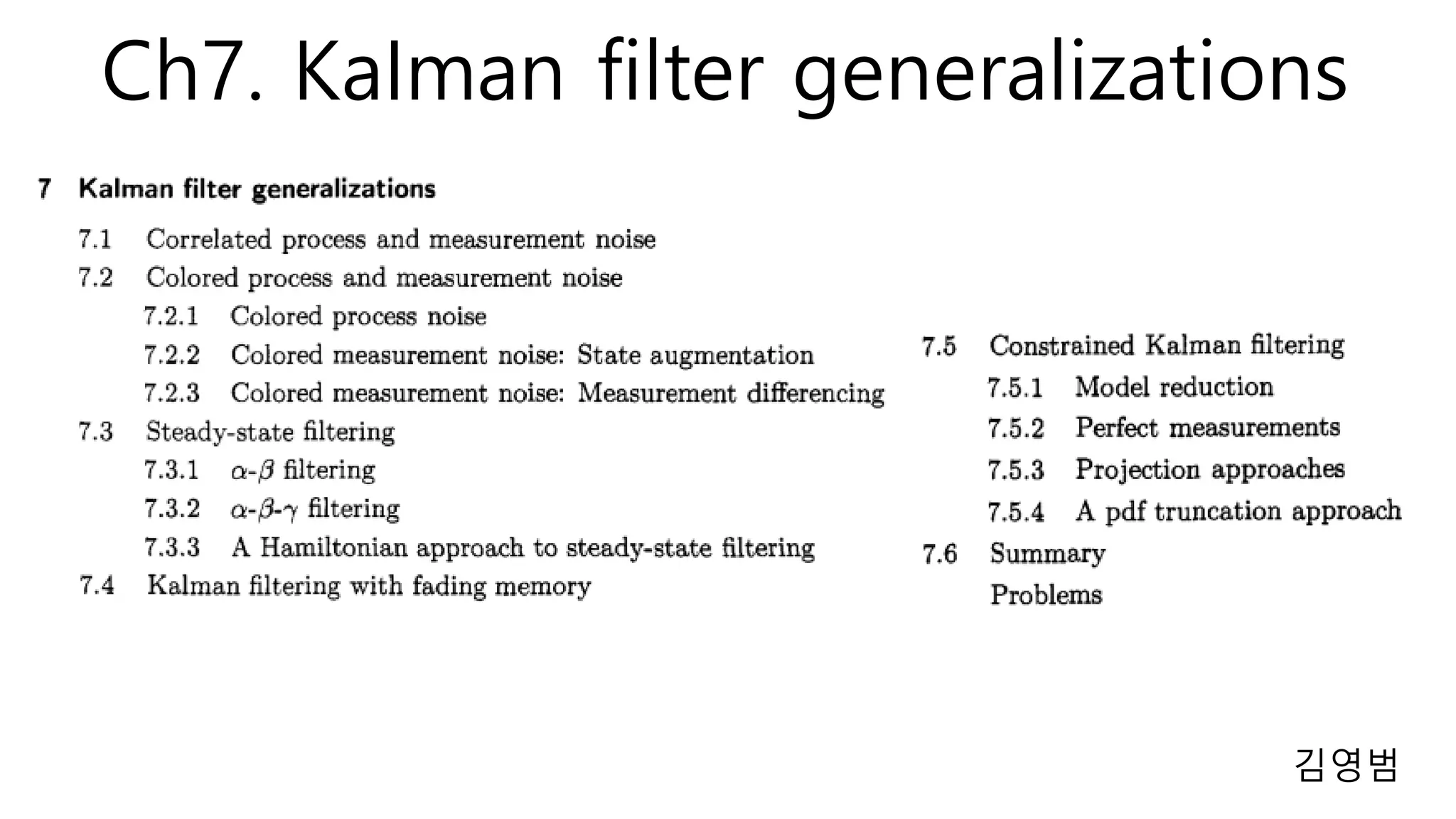
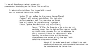
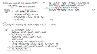
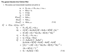
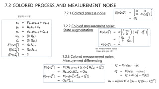
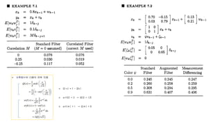
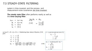
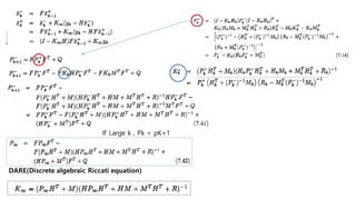
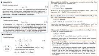
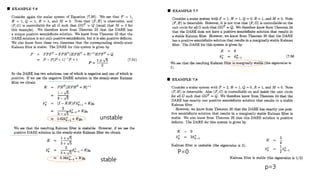
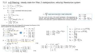
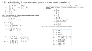
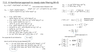
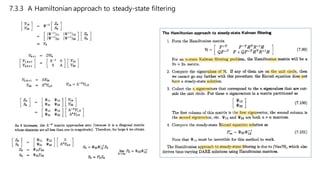
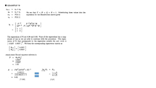
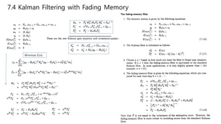
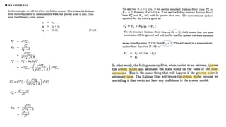
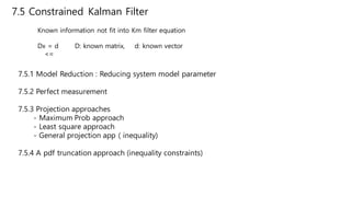
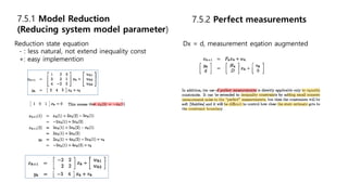
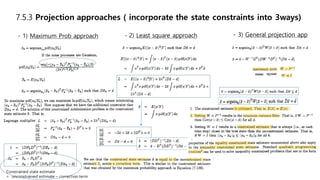
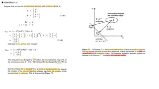
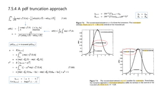
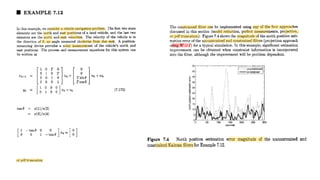
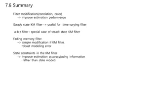
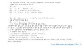
This document discusses several generalizations and modifications that can be made to the standard Kalman filter. Section 7.3 describes how a steady-state Kalman filter can be used instead of a time-varying filter when system dynamics are time-invariant. Section 7.4 discusses a fading memory filter that discounts older measurements to address cases when system dynamics are imperfectly known. Section 7.5 presents several approaches to incorporate state equality and inequality constraints into the Kalman filter formulation, including model reduction, projection approaches, and probability density function truncation.

1. Ch7. KaIman filter generalizations
김영범

2. Section 7.3 can replace the timevarying Kalman filter of
Chapter 5 with a steady-state Kalman filter that often
performs nearly as well. This means that we do not
have to compute the estimation-error covariance or
Kalman Optimal State Estimation, α-β, α-β-γ filtering
Section 7.4 When the dynamics of the system are not
perfectly known, then the Kalman filter may not provide
acceptable state estimates. This can be addressed by
giving more weight to recent measurements when
updating the state estimate, and discounting
measurements that arrived a long time ago. This is
called the fading-memory filter
Section 7.5 discusses several ways to incorporate state
equality constraints and state inequality constraints into
the formulation of the Kalman filter.
7.1, we will show how correlated process and
measurement noise changes the Kalman filter equations
7.2 We modify the Kalman filter to deal with colored
process noise and measurement noise

3. 7.1 CORRELATED PROCESS AND MEASUREMENT NOISE
how correlated process and measurement noise changes the Kalman filter equations.
We see that the process noise in the system equation is
correlated with the measurement noise, with the cross
covariance given by Mk6k-j+l.
In order to find the Kalman filter equations for the
correlated noise system, we will define the estimation
errors as

7. 7.2 COLORED PROCESS AND MEASUREMENT NOISE
7.2.1 Colored process noise
7.2.2 Colored measurement noise:
State augmentation
7.2.3 Colored measurement noise:
Measurement differencing
No measurement noise
mean and cov =0
일반적 시스템

9. 7.3 STEADY-STATE FILTERING
system is time-invariant, and the process- and
measurement-noise covariances are time-invariant,
The steady state filter often performs nearly as well as
the time-varying filter.

10. If Large k , Pk = pK+1
DARE(Discrete algebraic Riccati equation)

11. DARE

12. unstable
stable
P=0
p=3

13. 7.3.1 α-β filtering : steady state km filter, 2 state(position, velocity) Newtonian system

14. 7.3.2 α-β-γ filtering: 3 state Newtonian system( position, velocity, accelation)

15. 7.3.3 A Hamiltonian approach to steady-state filtering (M=0)

16. 7.3.3 A Hamiltonian approach to steady-state filtering

18. 7.4 Kalman Filtering with Fading Memory
Minimize E(Jn)

20. 7.5 Constrained Kalman Filter
Known information not fit into Km filter equation
Dx = d D: known matrix, d: known vector
<=
7.5.1 Model Reduction : Reducing system model parameter
7.5.2 Perfect measurement
7.5.3 Projection approaches
- Maximum Prob approach
- Least square approach
- General projection app ( inequality)
7.5.4 A pdf truncation approach (inequality constraints)

21. Reduction state equation
- : less natural, not extend inequality const
+: easy implemention
7.5.1 Model Reduction
(Reducing system model parameter)
7.5.2 Perfect measurements
Dx = d, measurement eqation augmented

22. - 1) Maximum Prob approach
7.5.3 Projection approaches ( incorporate the state constraints into 3ways)
- 2) Least square approach - 3) General projection app
Constrained state estimate
= unconstrained estimate – correction term

24. 7.5.4 A pdf truncation approach

26. 7.6 Summary
Filter modification(correlation, color)
-> improve estimation performence
Steady state KM filter -> useful for time varying filter
a-b-r filter : special case of steadt state KM filter
Fading memory filter
–> simple modification if KM filter,
robust modeling error
State constraints in the KM filter
-> improve estimation accuracy(using information
rather than state model)

27. https://blog.naver.com/lydsuper/38620339