The document discusses the extended Kalman filter (EKF), which extends the standard Kalman filter to nonlinear systems through linearization. The EKF linearizes the system equations at each time step by taking the derivative of the nonlinear functions around the current state estimate. This results in an approximate linear system that can then be processed using the standard Kalman filter equations. The key steps of the EKF algorithm are to 1) compute the linearized system matrices using derivatives, 2) use these in a first-order Taylor approximation to linearize the system equations, and 3) apply the standard Kalman filter equations to this approximate linear system to recursively estimate the state.

1. THE EXTENDED KALMAN FILTER
The Kalman filtering problem considered up to this point has addressed the estimation of as state vector
in a linear model of a dynamical system. If, however, the model is nonlinear, we may extend the use of
Kalman filteringthrough a linearizationprocedure. The resulting filter is naturally referred to as extended
Kalman filter (EFK). Such an extension is feasible by virtue of fact that Kalman filters described in terms
of differential equations (in the case of continuous–time systems) or difference equations (in the case of
discrete-time systems). This is in contrast to Wiener filter that is limited to linearsystems,since the
notion of an impulse response (on which the Wiener filter is based ) is meaningful only in the context of
linear systems . Hereis another important advantage of Kalman filter over the Wiener filter.
To set the stage for development of the extended Kalman filter in the discrete-time domain, consider
first the standard linear state –space model that we studied in the earlier part of this chapter [Eqs. (7.17)
and (7.19)], reproduced here for convenience of presentation:
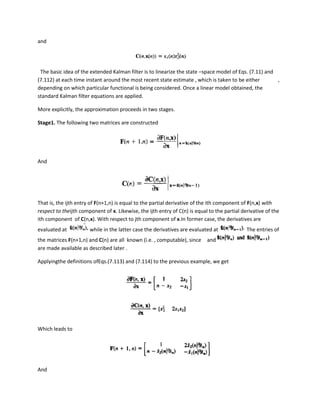
Where v1(n) and v2(n) are uncorrelated zero-mean white-noise processes with correlation matrices
Q1(n) and Q2(n), respectively, as defined in equations(7.18),(7.20), and (7.21). thecorresponding Kalman
filter equations are summarized in Table. In this section, however we will rewrite these equations in a
slightly modified form that is more convenient for our present discussion. Specifically,the update of the
sate estimate is performed in two steps . The first step updates this update
equation is simply (7.59).The second step updates and is obtained by substituting Eq.
(7.45)into Eq. (7.60),and by defining a new gain matrix:
We may thus write
We next make the following observation. Suppose thatinstead of the state equations (7.99) and (7.100),
weare given the alternative state vector model

2. Whered(n) is a known (i.e., nonrandom)vector . In this case, it is easily verified that the same Kalman
equations (7.103) through (7.107) apply except for a modification in the first equation (7.102)), which
now reads as follows
This modification arises in the derivation of extended Kalmanfilter, as discussed in the sequel.
As mentioned previously, the extended Kalman filter is an approximate solution that allows us to
extend the Kalman filtering idea to anonlinear state space models (Jazwimski, 1970 ;Maybeck,
1982;Lung and Soderstorm, 1983). In particular, the non-linear model considered here has the following
form:
Where,as before,v1 (n) and v2 (n) are uncorrelated zero-mean white–noise processes with correlation
matrices Q1(n) and Q2 (n) respectively. Here, however, the functionalF(n,x(n))denotes a nonlinear
transition matrix function that is not possibly time-variant. In the linear case, we simply have
But in a general nonlinear setting, the entriesof the state vector x(n) may combined nonlinearly by the
action of the functional; F(n.x (n) ).Moreover, this nonlinear operation may vary with time. Likewise, the
functional C(n, x(n))) denotes a nonlinear measurement matrix that may be time – variant too.
As an example, consider the following two-dimensional nonlinear state – space model:
In this example, we have

3. and
The basic idea of the extended Kalman filter is to linearize the state –space model of Eqs. (7.11) and
(7.112) at each time instant around the most recent state estimate , which is taken to be either ,
depending on which particular functional is being considered. Once a linear model obtained, the
standard Kalman filter equations are applied.
More explicitly, the approximation proceeds in two stages.
Stage1. The following two matrices are constructed
And
That is, the ijth entry of F(n+1,n) is equal to the partial derivative of the ith component of F(n,x) with
respect to theijth component of x. Likewise, the ijth entry of C(n) is equal to the partial derivative of the
ith component of C(n,x). With respect to jth component of x.In former case, the derivatives are
evaluated at while in the latter case the derivatives are evaluated at The entries of
the matrices F(n+1,n) and C(n) are all known (i.e. , computable), since and
are made available as described later .
Applyingthe definitions ofEqs.(7.113) and (7.114) to the previous example, we get
Which leads to
And

4. Stage 2.Once the matrices F(n+1,n) and C(n) are evaluated , they are then employed in a first- order
Taylor approximation of the nonlinear functionalF(n,x(n))and C(n,x(n)) around
and respectively. Specifically, F(n,x(n)) and C(n,x(n)) are approximated as follows,respectively :
With the above approximation expressions at hand, we may now proceed to approximate the nonlinear
state-equations (7.111) and (7.112) as shown by, respectively,
Where we have introduced two new quantities:
And
The entries in the term are known at time n, and, therefore, can be regarded as an
observationvector at timen. Likewise, the entries in the term d(n) are all known at time n.
Figure7.6. One-step predictor for the extended Kalman filter.

5. The approximate state-space model of Eqs.( 7.117) and (7.118) is a linear model of the same
mathematic al form as that described in Eqs. (7.108) and (7.109); indeed, it is with this objective in mind
that earlier on we formulated the state–space model of Eqs. (7.108)standard Kalman equations (7.13)
through (7.109) and (7.110) to the above linear model. This leads to the following set of equations:
On the basis of Eqs.(7.121) and (7.122), we may formulate the signal flow graph of Fig 7.6 for updating
the one-step prediction in the extended Kalman filter.
In table 7.5 we present a summary of the extended Kalman filtering algorithm, where the linearized
matricesF(n+1,n) and C(n) are computed from their respective nonlinear counterparts using Eqs.7.113
and (7.114). Given a nonlinear state- space model of the form described in Eqs. (7.111)and(7.112), we
may thus use this algorithm to compute state estimate recursively. Comparing the equations of the
extended Kalman filter summarized here in with those of the standard Kalman filter given Eqs.7.102

6. Table7.5 Summary of extended Kalman filter
through (7.107) we see that the only difference between them arise in the computations of the
innovcatiopns vector nad the updated estimate Specifically, the linear terms
in the standard Kalman filter are replaced by the approximate terms
respectively , in the extended Kalman filter . These differences also in
the standard Kalman gfilter with that of Fig7.6 for one-step prediction in the extended Kalman filter.