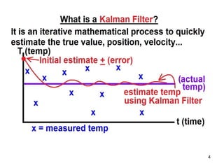
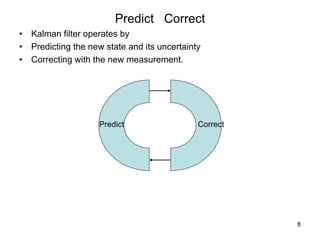
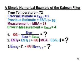
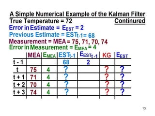
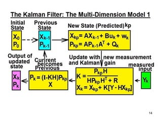
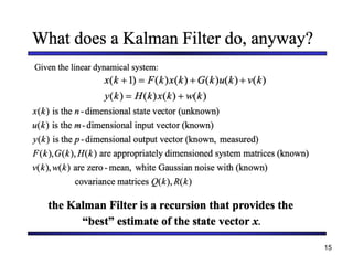
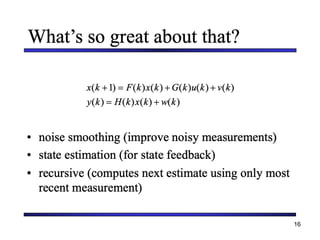
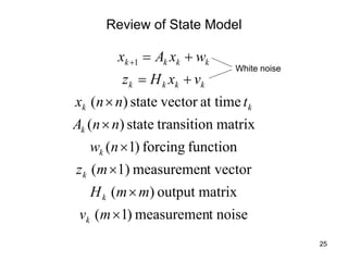
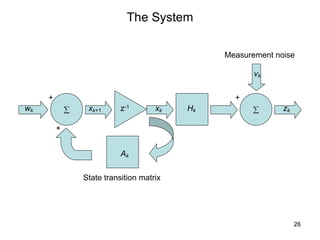
The Kalman filter is a mathematical algorithm that uses a series of measurements observed over time, containing statistical noise and other inaccuracies, and produces estimates of unknown variables that tend to be more precise than those based on a single measurement alone. It is effective at combining noisy sensor outputs to estimate the state of a dynamic system. Since its introduction in 1960, the Kalman filter has become widely used in applications like navigation systems, tracking objects, and computer vision. It works by predicting the new state and uncertainty, then correcting with a new measurement in a recursive manner.

1. 1
Kalman Filtering
• It is an effective and versatile mathematical procedure
for combining noisy sensor outputs to estimate the
state of a system with uncertain dynamics.
• Kalman filtering is a relatively recent (1960)
development in filtering.

2. 2
Kalman Filtering
Kalman filtering has been applied in areas as diverse as
• Aerospace,
• Tracking missiles,
• Navigation,
• Nuclear power plant instrumentation,
• Demographic modeling,
• Manufacturing,
• Computer vision applications.
For Kalman filter the problem formulated is state space
and is time varying.

3. 3
What is Kalman filter
Some Applied Math
Noisy data Less noisy data
Delay is the price for filtering

4. 4

5. 5
• The Kalman filter is a linear, recursive estimator that
produces the minimum variance estimate in a least
squares sense under the assumption of white,
Gaussian noise processes.
• Consider the problem of estimating the variables of a
system.
• In dynamic systems (that is, systems which vary
with time) the system variables are often denoted
by the term "state variables".
Since its introduction in 1960, the Kalman filter has become an integral
component in thousands of military and civilian navigation systems.

6. 6
• The Kalman filter is a multiple-input, multiple-
output digital filter that can optimally estimate, in
real time, the states of a system based on its noisy
outputs.
• The purpose of a Kalman filter is to estimate the state
of a system from measurements which contain
random errors.

7. 7
• An example is estimating the position and velocity of
a satellite from radar data.
• There are 3 components of position and 3 of velocity
so there are at least 6 variables to estimate.
• These variables are called state variables.
• With 6 state variables the resulting Kalman filter is
called a 6-dimensional Kalman filter.
To provide current estimates of the system variables - such as
position coordinates - the filter uses statistical models to properly
weight each new measurement relative to past information.

8. 8
Predict Correct
• Kalman filter operates by
• Predicting the new state and its uncertainty
• Correcting with the new measurement.
Predict Correct

9. 9

10. 10

11. 11

12. 12

13. 13

14. 14

15. 15

16. 16

17. 17

18. 18
Example: Two-dimensional Position Only
Process Model
k
k
k
k
k
k
k
k
k
k
k
k
k
w
x
A
x
w
x
A
x
y
x
y
x
y
x
+
=
+
=
ú
û
ù
ê
ë
é
+
ú
û
ù
ê
ë
é
ú
û
ù
ê
ë
é
=
ú
û
ù
ê
ë
é
+
-
-
-
-
-
-
1
1
1
1
1
1
1
Or
~
~
1
0
0
1
Noise
Noise
State State transition

19. 19
Measurement Model
k
v
k
x
H
k
z
k
v
k
u
k
y
k
x
y
H
x
H
k
v
k
u
+
=
ú
û
ù
ê
ë
é
+
ú
û
ù
ê
ë
é
ú
ú
û
ù
ê
ê
ë
é
=
ú
û
ù
ê
ë
é
~
~
0
0
Noise
Nose
measurement Measurement matrix

20. 20
Preparation
{ }
{ } Covariance
Noise
t
Measuremen
0
0
Covariance
Noise
Process
yy
Q
0
0
Transition
State
1
0
0
1
ú
ú
û
ù
ê
ê
ë
é
=
*
=
ú
ú
û
ù
ê
ê
ë
é
=
*
=
ú
û
ù
ê
ë
é
=
yy
R
xx
R
T
v
v
E
R
xx
Q
T
w
w
E
Q
A

21. 21
Initialization
ú
û
ù
ê
ë
é
=
=
e
e
0
0
o
P
o
z
H
o
x

22. 22
Predict
Q
T
A
k
AP
k
P
k
x
A
k
x
+
-
=
-
-
=
-
1
1
Uncertainty
Transition

23. 23
Correct
( )
1
-
÷
ø
ö
ç
è
æ +
-
-
=
-
-
=
÷
ø
ö
ç
è
æ -
-
+
-
=
R
T
H
k
HP
T
H
k
P
K
k
P
KH
I
k
P
k
x
H
k
z
K
k
x
k
x
Predicted
Actual
Measurement space

24. 24
Summary
Q
T
A
k
AP
k
P
k
x
A
k
x
+
-
=
-
-
=
-
1
1
( ) -
-
=
-
-
+
-
=
-
ú
û
ù
ê
ë
é +
-
-
=
k
P
KH
I
k
P
k
x
H
k
z
K
k
x
k
x
R
T
H
k
HP
T
H
k
P
K
)
(
1

25. 25
Review of State Model
noise
t
measuremen
)
1
(
matrix
output
)
(
t vector
measuremen
1)
(
function
forcing
)
1
(
matrix
n
transitio
state
)
(
at time
vector
state
)
(
1
´
´
´
´
´
´
+
=
+
=
+
m
v
m
m
H
m
z
n
w
n
n
A
t
n
n
x
v
x
H
z
w
x
A
x
k
k
k
k
k
k
k
k
k
k
k
k
k
k
k
White noise

26. 26
The System
å å
wk xk+1 z-1 xk Hk
vk
zk
Ak
+
+ +
Measurement noise
State transition matrix

27. 27
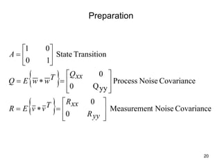
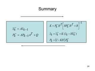
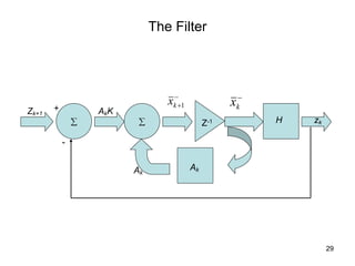
Kalman Predictor Update Equation
( )
[ ]
-
-
-
+ -
+
=
= k
k
k
k
k x
H
z
K
x
A
x
A
x 1
Prior estimate of xk
system.
actual
the
like
much
looks
that
system
a
be
out to
turn
will
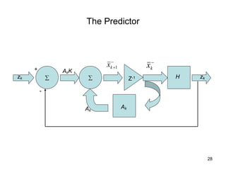
predictor
The

28. 28
The Predictor
-
k
x
å
zk
AkK
zk
Ak
-
+
å H
Ak
Z-1
-
+1
k
x

29. 29
The Filter
-
k
x
å
Zk+1 AkK
zk
Ak
-
+
å H
Ak
Z-1
-
+1
k
x

30. 30
How Kalman Filter Works?
• The Kalman filter maintains two types of variables:
• Estimate State Vector: The components of the estimated state
vector include the following:
– The variables of interest (what we want or need to know, such as
position and velocity).
– Nuisance variables that may be necessary to the estimation process.
– The Kalman filter state variables for a specific application must include
all those system dynamic variables that are measurable by the sensors
used in the application.
• A Covariance Matrix: a measure of estimation uncertainty. The
equations used to propagate the covariance matrix (collectively
called the Riccati equation) model and manage uncertainty, taking
into account how sensor noise and dynamic uncertainty contribute to
uncertainty about the estimated system state.

31. 31
• By maintaining an estimate of its own estimation uncertainty and the
relative uncertainty in the various sensor outputs, the Kalman filter is
able to combine all sensor information “optimally” in the sense that
the resulting estimate minimizes any quadratic loss function of
estimation, including the mean-squared value of any linear
combination of static estimation errors.
• The Kalman gain is the optimal weighting matrix for combining new
sensor data with a prior estimate to obtain a new estimate.