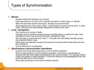
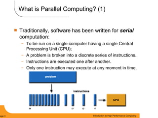
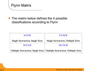
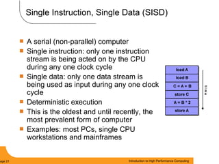
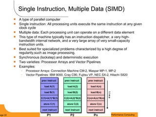
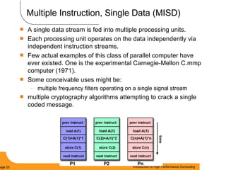
This document provides an introduction to parallel computing. It begins with definitions of parallel computing as using multiple compute resources simultaneously to solve problems. Popular parallel architectures include shared memory, where all processors can access a common memory, and distributed memory, where each processor has its own local memory and they communicate over a network. The document discusses key parallel computing concepts and terminology such as Flynn's taxonomy, parallel overhead, scalability, and memory models including uniform memory access (UMA), non-uniform memory access (NUMA), and distributed memory. It aims to provide background on parallel computing topics before examining how to parallelize different types of programs.
Parallel computing and its applicationsBurhan Ahmed
Parallel computing is a type of computing architecture in which several processors execute or process an application or computation simultaneously. Parallel computing helps in performing large computations by dividing the workload between more than one processor, all of which work through the computation at the same time. Most supercomputers employ parallel computing principles to operate. Parallel computing is also known as parallel processing.
↓↓↓↓ Read More:
Watch my videos on snack here: --> --> http://sck.io/x-B1f0Iy
@ Kindly Follow my Instagram Page to discuss about your mental health problems-
-----> https://instagram.com/mentality_streak?utm_medium=copy_link
@ Appreciate my work:
-----> behance.net/burhanahmed1
Thank-you !
The primary reasons for using parallel computing:
Save time - wall clock time
Solve larger problems
Provide concurrency (do multiple things at the same time)
Please contact me to download this pres.A comprehensive presentation on the field of Parallel Computing.It's applications are only growing exponentially day by days.A useful seminar covering basics,its classification and implementation thoroughly.
Visit www.ameyawaghmare.wordpress.com for more info
program partitioning and scheduling IN Advanced Computer ArchitecturePankaj Kumar Jain
Advanced Computer Architecture,Program Partitioning and Scheduling,Program Partitioning & Scheduling,Latency,Levels of Parallelism,Loop-level Parallelism,Subprogram-level Parallelism,Job or Program-Level Parallelism,Communication Latency,Grain Packing and Scheduling,Program Graphs and Packing
In this presentation, you will learn the fundamentals of Multi Processors and Multi Computers in only a few minutes.
Meanings, features, attributes, applications, and examples of multiprocessors and multi computers.
So, let's get started. If you enjoy this and find the information beneficial, please like and share it with your friends.
A multi-core processor is a single computing component with two or more independent actual processing units (called "cores"), which are units that read and execute program instructions. The instructions are ordinary CPU instructions (such as add, move data, and branch), but the multiple cores can run multiple instructions at the same time, increasing overall speed for programs amenable to parallel computing. Manufacturers typically integrate the cores onto a single integrated circuit die (known as a chip multiprocessor or CMP), or onto multiple dies in a single chip package.
Parallel computing is computing architecture paradigm ., in which processing required to solve a problem is done in more than one processor parallel way.
advanced computer architesture-conditions of parallelismPankaj Kumar Jain
This PPT contains Data and Resource Dependencies,Control Dependence,Resource Dependence,Bernstein’s Conditions ,Hardware And Software Parallelism,Types of Software Parallelism
Parallel computing diu pi cluster by Prof. Dr. Syed Akhter Hossain & Md SamiMD Sami
DIU Pi cluster is a new generation cluster technology. It’s a prototype project power by Raspberry Pi . we design a very low cost cluster with low cost hardware and equipment. DIU Pi cluster is build for serve multi purpose Technology Like Big Data , Parallel processing,
Medical image processing and also for Artificial intelligence (AI) implementation
Highly Surmountable Challenges in Ruby+OMR JIT CompilationMatthew Gaudet
The Ruby+OMR JIT compiler adds a JIT to CRuby. However, it has challenges to surmount before it will provide broad improvement to Ruby applications that aren’t micro-benchmarks. This talk will cover some of those challenges, along with some brainstorming about potential ways to tackle them.
The Ruby+OMR JIT compiler is one way to add JIT compilation to the CRuby interpreter. However, it has a number of challenges to surmount before it will provide broad improvement to Ruby applications that aren’t micro-benchmarks. This talk will cover some of those challenges, along with some brainstorming about potential ways to tackle them.
Parallel computing is a type of computation in which many calculations or the execution of processes are carried out simultaneously. Large problems can often be divided into smaller ones, which can then be solved at the same time. There are several different forms of parallel computing: bit-level, instruction-level, data, and task parallelism. Parallelism has been employed for many years, mainly in high-performance computing, but interest in it has grown lately due to the physical constraints preventing frequency scaling. As power consumption (and consequently heat generation) by computers has become a concern in recent years, parallel computing has become the dominant paradigm in computer architecture, mainly in the form of multi-core processors.
For over 40 years, virtually all computers have followed a common machine model known as the von Neumann computer. Name after the Hungarian mathématicien John von Neumann.
A von Neumann computer uses the stored-program concept. The CPU executes a stored program that specifies a sequence of read and write operations on the memory.
Today, We will discuss about the "Introduction to Parallel Computing". This slides design very simple and easy, you can easily understand of this slide, if you have any query please ping me, i will be the answer quickly.
This Chapter provides a Background Review of Parallel and Distributed Computing. a focus is made on the concept of SISD, SIMD, MISD, MIMD.
It also gives an understanding of the notion of HPC (High-Performance Computing). A survey is done using some case studies to show why parallelism is needed. The chapter discusses the Amdahl's Law and the limitations. Gustafson's Law is also discussed.
This is my report in MIS at PNU MA class. All the materials (e.g.text, graphics, images) I used were downloaded from the net. I just came up for some important details and proceeded with the presentation..
This chapter discusses various classification attributed to parallel architectures. It also introduces related parallel programming models and presents the actions of these models on parallel architectures. Notions such as Data parallelism Task parallelism, Tighty and Coupled system, UMA/NUMA, Multicore computing, Symmetric multiprocessing, Distributed Computing, Cluster computing, Shared memory without thread/Thread, etc..
Operation “Blue Star” is the only event in the history of Independent India where the state went into war with its own people. Even after about 40 years it is not clear if it was culmination of states anger over people of the region, a political game of power or start of dictatorial chapter in the democratic setup.
The people of Punjab felt alienated from main stream due to denial of their just demands during a long democratic struggle since independence. As it happen all over the word, it led to militant struggle with great loss of lives of military, police and civilian personnel. Killing of Indira Gandhi and massacre of innocent Sikhs in Delhi and other India cities was also associated with this movement.
June 3, 2024 Anti-Semitism Letter Sent to MIT President Kornbluth and MIT Cor...Levi Shapiro
Letter from the Congress of the United States regarding Anti-Semitism sent June 3rd to MIT President Sally Kornbluth, MIT Corp Chair, Mark Gorenberg
Dear Dr. Kornbluth and Mr. Gorenberg,
The US House of Representatives is deeply concerned by ongoing and pervasive acts of antisemitic
harassment and intimidation at the Massachusetts Institute of Technology (MIT). Failing to act decisively to ensure a safe learning environment for all students would be a grave dereliction of your responsibilities as President of MIT and Chair of the MIT Corporation.
This Congress will not stand idly by and allow an environment hostile to Jewish students to persist. The House believes that your institution is in violation of Title VI of the Civil Rights Act, and the inability or
unwillingness to rectify this violation through action requires accountability.
Postsecondary education is a unique opportunity for students to learn and have their ideas and beliefs challenged. However, universities receiving hundreds of millions of federal funds annually have denied
students that opportunity and have been hijacked to become venues for the promotion of terrorism, antisemitic harassment and intimidation, unlawful encampments, and in some cases, assaults and riots.
The House of Representatives will not countenance the use of federal funds to indoctrinate students into hateful, antisemitic, anti-American supporters of terrorism. Investigations into campus antisemitism by the Committee on Education and the Workforce and the Committee on Ways and Means have been expanded into a Congress-wide probe across all relevant jurisdictions to address this national crisis. The undersigned Committees will conduct oversight into the use of federal funds at MIT and its learning environment under authorities granted to each Committee.
• The Committee on Education and the Workforce has been investigating your institution since December 7, 2023. The Committee has broad jurisdiction over postsecondary education, including its compliance with Title VI of the Civil Rights Act, campus safety concerns over disruptions to the learning environment, and the awarding of federal student aid under the Higher Education Act.
• The Committee on Oversight and Accountability is investigating the sources of funding and other support flowing to groups espousing pro-Hamas propaganda and engaged in antisemitic harassment and intimidation of students. The Committee on Oversight and Accountability is the principal oversight committee of the US House of Representatives and has broad authority to investigate “any matter” at “any time” under House Rule X.
• The Committee on Ways and Means has been investigating several universities since November 15, 2023, when the Committee held a hearing entitled From Ivory Towers to Dark Corners: Investigating the Nexus Between Antisemitism, Tax-Exempt Universities, and Terror Financing. The Committee followed the hearing with letters to those institutions on January 10, 202
Macroeconomics- Movie Location
This will be used as part of your Personal Professional Portfolio once graded.
Objective:
Prepare a presentation or a paper using research, basic comparative analysis, data organization and application of economic information. You will make an informed assessment of an economic climate outside of the United States to accomplish an entertainment industry objective.
Introduction to AI for Nonprofits with Tapp NetworkTechSoup
Dive into the world of AI! Experts Jon Hill and Tareq Monaur will guide you through AI's role in enhancing nonprofit websites and basic marketing strategies, making it easy to understand and apply.
Welcome to TechSoup New Member Orientation and Q&A (May 2024).pdfTechSoup
In this webinar you will learn how your organization can access TechSoup's wide variety of product discount and donation programs. From hardware to software, we'll give you a tour of the tools available to help your nonprofit with productivity, collaboration, financial management, donor tracking, security, and more.
The French Revolution, which began in 1789, was a period of radical social and political upheaval in France. It marked the decline of absolute monarchies, the rise of secular and democratic republics, and the eventual rise of Napoleon Bonaparte. This revolutionary period is crucial in understanding the transition from feudalism to modernity in Europe.
For more information, visit-www.vavaclasses.com
A Strategic Approach: GenAI in EducationPeter Windle
Artificial Intelligence (AI) technologies such as Generative AI, Image Generators and Large Language Models have had a dramatic impact on teaching, learning and assessment over the past 18 months. The most immediate threat AI posed was to Academic Integrity with Higher Education Institutes (HEIs) focusing their efforts on combating the use of GenAI in assessment. Guidelines were developed for staff and students, policies put in place too. Innovative educators have forged paths in the use of Generative AI for teaching, learning and assessments leading to pockets of transformation springing up across HEIs, often with little or no top-down guidance, support or direction.
This Gasta posits a strategic approach to integrating AI into HEIs to prepare staff, students and the curriculum for an evolving world and workplace. We will highlight the advantages of working with these technologies beyond the realm of teaching, learning and assessment by considering prompt engineering skills, industry impact, curriculum changes, and the need for staff upskilling. In contrast, not engaging strategically with Generative AI poses risks, including falling behind peers, missed opportunities and failing to ensure our graduates remain employable. The rapid evolution of AI technologies necessitates a proactive and strategic approach if we are to remain relevant.
2. Introduction to High Performance ComputingPage 2
Abstract
This presentation covers the basics of parallel computing.
Beginning with a brief overview and some concepts and
terminology associated with parallel computing, the topics of
parallel memory architectures and programming models are
then explored. These topics are followed by a discussion on a
number of issues related to designing parallel programs. The
last portion of the presentation is spent examining how to
parallelize several different types of serial programs.
Level/Prerequisites: None
3. Introduction to High Performance ComputingPage 3
What is Parallel Computing? (1)
Traditionally, software has been written for serial
computation:
– To be run on a single computer having a single Central
Processing Unit (CPU);
– A problem is broken into a discrete series of instructions.
– Instructions are executed one after another.
– Only one instruction may execute at any moment in time.
4. Introduction to High Performance ComputingPage 4
What is Parallel Computing? (2)
In the simplest sense, parallel computing is the simultaneous use of
multiple compute resources to solve a computational problem.
– To be run using multiple CPUs
– A problem is broken into discrete parts that can be solved concurrently
– Each part is further broken down to a series of instructions
Instructions from each part execute simultaneously on different CPUs
5. Introduction to High Performance ComputingPage 5
Parallel Computing: Resources
The compute resources can include:
– A single computer with multiple processors;
– A single computer with (multiple) processor(s) and some
specialized computer resources (GPU, FPGA …)
– An arbitrary number of computers connected by a network;
– A combination of both.
6. Introduction to High Performance ComputingPage 6
Parallel Computing: The computational problem
The computational problem usually demonstrates
characteristics such as the ability to be:
– Broken apart into discrete pieces of work that can be solved
simultaneously;
– Execute multiple program instructions at any moment in
time;
– Solved in less time with multiple compute resources than
with a single compute resource.
7. Introduction to High Performance ComputingPage 7
Parallel Computing: what for? (1)
Parallel computing is an evolution of serial computing that
attempts to emulate what has always been the state of affairs in
the natural world: many complex, interrelated events happening
at the same time, yet within a sequence.
Some examples:
– Planetary and galactic orbits
– Weather and ocean patterns
– Tectonic plate drift
– Rush hour traffic in Paris
– Automobile assembly line
– Daily operations within a business
– Building a shopping mall
– Ordering a hamburger at the drive through.
8. Introduction to High Performance ComputingPage 8
Parallel Computing: what for? (2)
Traditionally, parallel computing has been considered
to be "the high end of computing" and has been
motivated by numerical simulations of complex
systems and "Grand Challenge Problems" such as:
– weather and climate
– chemical and nuclear reactions
– biological, human genome
– geological, seismic activity
– mechanical devices - from prosthetics to spacecraft
– electronic circuits
– manufacturing processes
9. Introduction to High Performance ComputingPage 9
Parallel Computing: what for? (3)
Today, commercial applications are providing an equal or
greater driving force in the development of faster computers.
These applications require the processing of large amounts of
data in sophisticated ways. Example applications include:
– parallel databases, data mining
– oil exploration
– web search engines, web based business services
– computer-aided diagnosis in medicine
– management of national and multi-national corporations
– advanced graphics and virtual reality, particularly in the
entertainment industry
– networked video and multi-media technologies
– collaborative work environments
Ultimately, parallel computing is an attempt to maximize the
infinite but seemingly scarce commodity called time.
10. Introduction to High Performance ComputingPage 10
Why Parallel Computing? (1)
This is a legitime question! Parallel computing is
complex on any aspect!
The primary reasons for using parallel computing:
– Save time - wall clock time
– Solve larger problems
– Provide concurrency (do multiple things at the same time)
11. Introduction to High Performance ComputingPage 11
Why Parallel Computing? (2)
Other reasons might include:
– Taking advantage of non-local resources - using available
compute resources on a wide area network, or even the
Internet when local compute resources are scarce.
– Cost savings - using multiple "cheap" computing resources
instead of paying for time on a supercomputer.
– Overcoming memory constraints - single computers have
very finite memory resources. For large problems, using the
memories of multiple computers may overcome this
obstacle.
12. Introduction to High Performance ComputingPage 12
Limitations of Serial Computing
Limits to serial computing - both physical and practical reasons pose
significant constraints to simply building ever faster serial computers.
Transmission speeds - the speed of a serial computer is directly
dependent upon how fast data can move through hardware. Absolute
limits are the speed of light (30 cm/nanosecond) and the transmission
limit of copper wire (9 cm/nanosecond). Increasing speeds necessitate
increasing proximity of processing elements.
Limits to miniaturization - processor technology is allowing an
increasing number of transistors to be placed on a chip. However, even
with molecular or atomic-level components, a limit will be reached on
how small components can be.
Economic limitations - it is increasingly expensive to make a single
processor faster. Using a larger number of moderately fast commodity
processors to achieve the same (or better) performance is less
expensive.
13. Introduction to High Performance ComputingPage 13
The future
during the past 10 years, the trends indicated by ever
faster networks, distributed systems, and multi-
processor computer architectures (even at the
desktop level) clearly show that parallelism is the
future of computing.
It will be multi-forms, mixing general purpose
solutions (your PC…) and very speciliazed solutions
as IBM Cells, ClearSpeed, GPGPU from NVidia …
14. Introduction to High Performance ComputingPage 14
Who and What? (1)
Top500.org provides statistics on parallel computing
users - the charts below are just a sample. Some
things to note:
– Sectors may overlap - for example, research may be
classified research. Respondents have to choose between
the two.
"Not Specified" is by far the largest application -
probably means multiple applications.
17. Introduction to High Performance ComputingPage 17
Von Neumann Architecture
For over 40 years, virtually all computers have
followed a common machine model known as the von
Neumann computer. Named after the Hungarian
mathematician John von Neumann.
A von Neumann computer uses the stored-program
concept. The CPU executes a stored program that
specifies a sequence of read and write operations on
the memory.
18. Introduction to High Performance ComputingPage 18
Basic Design
Basic design
– Memory is used to store both
program and data instructions
– Program instructions are coded data
which tell the computer to do
something
– Data is simply information to be used
by the program
A central processing unit (CPU)
gets instructions and/or data from
memory, decodes the instructions
and then sequentially performs
them.
19. Introduction to High Performance ComputingPage 19
Flynn's Classical Taxonomy
There are different ways to classify parallel
computers. One of the more widely used
classifications, in use since 1966, is called Flynn's
Taxonomy.
Flynn's taxonomy distinguishes multi-processor
computer architectures according to how they can be
classified along the two independent dimensions of
Instruction and Data. Each of these dimensions can
have only one of two possible states: Single or
Multiple.
20. Introduction to High Performance ComputingPage 20
Flynn Matrix
The matrix below defines the 4 possible
classifications according to Flynn
21. Introduction to High Performance ComputingPage 21
Single Instruction, Single Data (SISD)
A serial (non-parallel) computer
Single instruction: only one instruction
stream is being acted on by the CPU
during any one clock cycle
Single data: only one data stream is
being used as input during any one clock
cycle
Deterministic execution
This is the oldest and until recently, the
most prevalent form of computer
Examples: most PCs, single CPU
workstations and mainframes
22. Introduction to High Performance ComputingPage 22
Single Instruction, Multiple Data (SIMD)
A type of parallel computer
Single instruction: All processing units execute the same instruction at any given
clock cycle
Multiple data: Each processing unit can operate on a different data element
This type of machine typically has an instruction dispatcher, a very high-
bandwidth internal network, and a very large array of very small-capacity
instruction units.
Best suited for specialized problems characterized by a high degree of
regularity,such as image processing.
Synchronous (lockstep) and deterministic execution
Two varieties: Processor Arrays and Vector Pipelines
Examples:
– Processor Arrays: Connection Machine CM-2, Maspar MP-1, MP-2
– Vector Pipelines: IBM 9000, Cray C90, Fujitsu VP, NEC SX-2, Hitachi S820
23. Introduction to High Performance ComputingPage 23
Multiple Instruction, Single Data (MISD)
A single data stream is fed into multiple processing units.
Each processing unit operates on the data independently via
independent instruction streams.
Few actual examples of this class of parallel computer have
ever existed. One is the experimental Carnegie-Mellon C.mmp
computer (1971).
Some conceivable uses might be:
– multiple frequency filters operating on a single signal stream
multiple cryptography algorithms attempting to crack a single
coded message.
24. Introduction to High Performance ComputingPage 24
Multiple Instruction, Multiple Data (MIMD)
Currently, the most common type of parallel computer. Most
modern computers fall into this category.
Multiple Instruction: every processor may be executing a
different instruction stream
Multiple Data: every processor may be working with a different
data stream
Execution can be synchronous or asynchronous, deterministic
or non-deterministic
Examples: most current supercomputers, networked parallel
computer "grids" and multi-processor SMP computers -
including some types of PCs.
25. Introduction to High Performance ComputingPage 25
Some General Parallel Terminology
Task
– A logically discrete section of computational work. A task is
typically a program or program-like set of instructions that is
executed by a processor.
Parallel Task
– A task that can be executed by multiple processors safely
(yields correct results)
Serial Execution
– Execution of a program sequentially, one statement at a
time. In the simplest sense, this is what happens on a one
processor machine. However, virtually all parallel tasks will
have sections of a parallel program that must be executed
serially.
Like everything else, parallel computing has its own "jargon". Some of the
more commonly used terms associated with parallel computing are listed
below. Most of these will be discussed in more detail later.
26. Introduction to High Performance ComputingPage 26
Parallel Execution
– Execution of a program by more than one task, with each task
being able to execute the same or different statement at the same
moment in time.
Shared Memory
– From a strictly hardware point of view, describes a computer
architecture where all processors have direct (usually bus based)
access to common physical memory. In a programming sense, it
describes a model where parallel tasks all have the same "picture"
of memory and can directly address and access the same logical
memory locations regardless of where the physical memory actually
exists.
Distributed Memory
– In hardware, refers to network based memory access for physical
memory that is not common. As a programming model, tasks can
only logically "see" local machine memory and must use
communications to access memory on other machines where other
tasks are executing.
27. Introduction to High Performance ComputingPage 27
Communications
– Parallel tasks typically need to exchange data. There are several
ways this can be accomplished, such as through a shared memory
bus or over a network, however the actual event of data exchange
is commonly referred to as communications regardless of the
method employed.
Synchronization
– The coordination of parallel tasks in real time, very often associated
with communications. Often implemented by establishing a
synchronization point within an application where a task may not
proceed further until another task(s) reaches the same or logically
equivalent point.
– Synchronization usually involves waiting by at least one task, and
can therefore cause a parallel application's wall clock execution
time to increase.
28. Introduction to High Performance ComputingPage 28
Granularity
– In parallel computing, granularity is a qualitative measure of the
ratio of computation to communication.
– Coarse: relatively large amounts of computational work are done
between communication events
– Fine: relatively small amounts of computational work are done
between communication events
Observed Speedup
– Observed speedup of a code which has been parallelized, defined
as:
wall-clock time of serial execution
wall-clock time of parallel execution
– One of the simplest and most widely used indicators for a parallel
program's performance.
29. Introduction to High Performance ComputingPage 29
Parallel Overhead
– The amount of time required to coordinate parallel tasks, as
opposed to doing useful work. Parallel overhead can include factors
such as:
− Task start-up time
− Synchronizations
− Data communications
− Software overhead imposed by parallel compilers, libraries, tools,
operating system, etc.
− Task termination time
Massively Parallel
– Refers to the hardware that comprises a given parallel system -
having many processors. The meaning of many keeps increasing,
but currently BG/L pushes this number to 6 digits.
30. Introduction to High Performance ComputingPage 30
Scalability
– Refers to a parallel system's (hardware and/or software)
ability to demonstrate a proportionate increase in parallel
speedup with the addition of more processors. Factors that
contribute to scalability include:
− Hardware - particularly memory-cpu bandwidths and network
communications
− Application algorithm
− Parallel overhead related
− Characteristics of your specific application and coding
32. Introduction to High Performance ComputingPage 32
Memory architectures
Shared Memory
Distributed Memory
Hybrid Distributed-Shared Memory
33. Introduction to High Performance ComputingPage 33
Shared Memory
Shared memory parallel computers vary widely, but generally
have in common the ability for all processors to access all
memory as global address space.
Multiple processors can operate independently but share the
same memory resources.
Changes in a memory location effected by one processor are
visible to all other processors.
Shared memory machines can be divided into two main classes
based upon memory access times: UMA and NUMA.
34. Introduction to High Performance ComputingPage 34
Shared Memory : UMA vs. NUMA
Uniform Memory Access (UMA):
– Most commonly represented today by Symmetric Multiprocessor
(SMP) machines
– Identical processors
– Equal access and access times to memory
– Sometimes called CC-UMA - Cache Coherent UMA. Cache
coherent means if one processor updates a location in shared
memory, all the other processors know about the update. Cache
coherency is accomplished at the hardware level.
Non-Uniform Memory Access (NUMA):
– Often made by physically linking two or more SMPs
– One SMP can directly access memory of another SMP
– Not all processors have equal access time to all memories
– Memory access across link is slower
– If cache coherency is maintained, then may also be called CC-
NUMA - Cache Coherent NUMA
35. Introduction to High Performance ComputingPage 35
Shared Memory: Pro and Con
Advantages
– Global address space provides a user-friendly programming
perspective to memory
– Data sharing between tasks is both fast and uniform due to the
proximity of memory to CPUs
Disadvantages:
– Primary disadvantage is the lack of scalability between memory and
CPUs. Adding more CPUs can geometrically increases traffic on
the shared memory-CPU path, and for cache coherent systems,
geometrically increase traffic associated with cache/memory
management.
– Programmer responsibility for synchronization constructs that
insure "correct" access of global memory.
– Expense: it becomes increasingly difficult and expensive to design
and produce shared memory machines with ever increasing
numbers of processors.
36. Introduction to High Performance ComputingPage 36
Distributed Memory
Like shared memory systems, distributed memory systems vary widely but share
a common characteristic. Distributed memory systems require a communication
network to connect inter-processor memory.
Processors have their own local memory. Memory addresses in one processor
do not map to another processor, so there is no concept of global address space
across all processors.
Because each processor has its own local memory, it operates independently.
Changes it makes to its local memory have no effect on the memory of other
processors. Hence, the concept of cache coherency does not apply.
When a processor needs access to data in another processor, it is usually the
task of the programmer to explicitly define how and when data is communicated.
Synchronization between tasks is likewise the programmer's responsibility.
The network "fabric" used for data transfer varies widely, though it can can be as
simple as Ethernet.
37. Introduction to High Performance ComputingPage 37
Distributed Memory: Pro and Con
Advantages
– Memory is scalable with number of processors. Increase the
number of processors and the size of memory increases
proportionately.
– Each processor can rapidly access its own memory without
interference and without the overhead incurred with trying to
maintain cache coherency.
– Cost effectiveness: can use commodity, off-the-shelf processors
and networking.
Disadvantages
– The programmer is responsible for many of the details associated
with data communication between processors.
– It may be difficult to map existing data structures, based on global
memory, to this memory organization.
– Non-uniform memory access (NUMA) times
38. Introduction to High Performance ComputingPage 38
Hybrid Distributed-Shared Memory
Comparison of Shared and Distributed Memory Architectures
Architecture CC-UMA CC-NUMA Distributed
Examples SMPs
Sun Vexx
DEC/Compaq
SGI Challenge
IBM POWER3
Bull NovaScale
SGI Origin
Sequent
HP Exemplar
DEC/Compaq
IBM POWER4 (MCM)
Cray T3E
Maspar
IBM SP2
IBM BlueGene
Communications MPI
Threads
OpenMP
shmem
MPI
Threads
OpenMP
shmem
MPI
Scalability to 10s of processors to 100s of processors to 1000s of processors
Draw Backs Memory-CPU bandwidth Memory-CPU bandwidth
Non-uniform access
times
System administration
Programming is hard to
develop and maintain
Software Availability many 1000s ISVs many 1000s ISVs 100s ISVs
Summarizing a few of the key characteristics of shared and
distributed memory machines
39. Introduction to High Performance ComputingPage 39
Hybrid Distributed-Shared Memory
The largest and fastest computers in the world today employ both
shared and distributed memory architectures.
The shared memory component is usually a cache coherent SMP
machine. Processors on a given SMP can address that machine's
memory as global.
The distributed memory component is the networking of multiple SMPs.
SMPs know only about their own memory - not the memory on another
SMP. Therefore, network communications are required to move data
from one SMP to another.
Current trends seem to indicate that this type of memory architecture
will continue to prevail and increase at the high end of computing for
the foreseeable future.
Advantages and Disadvantages: whatever is common to both shared
and distributed memory architectures.
41. Introduction to High Performance ComputingPage 41
Overview
Shared Memory Model
Threads Model
Message Passing Model
Data Parallel Model
Other Models
42. Introduction to High Performance ComputingPage 42
Overview
There are several parallel programming models in
common use:
– Shared Memory
– Threads
– Message Passing
– Data Parallel
– Hybrid
Parallel programming models exist as an abstraction
above hardware and memory architectures.
43. Introduction to High Performance ComputingPage 43
Overview
Although it might not seem apparent, these models are NOT specific to
a particular type of machine or memory architecture. In fact, any of
these models can (theoretically) be implemented on any underlying
hardware.
Shared memory model on a distributed memory machine: Kendall
Square Research (KSR) ALLCACHE approach.
– Machine memory was physically distributed, but appeared to the user as a
single shared memory (global address space). Generically, this approach is
referred to as "virtual shared memory".
– Note: although KSR is no longer in business, there is no reason to suggest
that a similar implementation will not be made available by another vendor
in the future.
– Message passing model on a shared memory machine: MPI on SGI Origin.
The SGI Origin employed the CC-NUMA type of shared memory
architecture, where every task has direct access to global memory.
However, the ability to send and receive messages with MPI, as is
commonly done over a network of distributed memory machines, is not
only implemented but is very commonly used.
44. Introduction to High Performance ComputingPage 44
Overview
Which model to use is often a combination of what is
available and personal choice. There is no "best"
model, although there certainly are better
implementations of some models over others.
The following sections describe each of the models
mentioned above, and also discuss some of their
actual implementations.
45. Introduction to High Performance ComputingPage 45
Shared Memory Model
In the shared-memory programming model, tasks share a
common address space, which they read and write
asynchronously.
Various mechanisms such as locks / semaphores may be used
to control access to the shared memory.
An advantage of this model from the programmer's point of view
is that the notion of data "ownership" is lacking, so there is no
need to specify explicitly the communication of data between
tasks. Program development can often be simplified.
An important disadvantage in terms of performance is that it
becomes more difficult to understand and manage data locality.
46. Introduction to High Performance ComputingPage 46
Shared Memory Model: Implementations
On shared memory platforms, the native compilers
translate user program variables into actual memory
addresses, which are global.
No common distributed memory platform
implementations currently exist. However, as
mentioned previously in the Overview section, the
KSR ALLCACHE approach provided a shared
memory view of data even though the physical
memory of the machine was distributed.
47. Introduction to High Performance ComputingPage 47
Threads Model
In the threads model of parallel programming, a single process can have
multiple, concurrent execution paths.
Perhaps the most simple analogy that can be used to describe threads is the
concept of a single program that includes a number of subroutines:
– The main program a.out is scheduled to run by the native operating system. a.out
loads and acquires all of the necessary system and user resources to run.
– a.out performs some serial work, and then creates a number of tasks (threads) that
can be scheduled and run by the operating system concurrently.
– Each thread has local data, but also, shares the entire resources of a.out. This
saves the overhead associated with replicating a program's resources for each thread.
Each thread also benefits from a global memory view because it shares the memory
space of a.out.
– A thread's work may best be described as a subroutine within the main program. Any
thread can execute any subroutine at the same time as other threads.
– Threads communicate with each other through global memory (updating address
locations). This requires synchronization constructs to insure that more than one
thread is not updating the same global address at any time.
– Threads can come and go, but a.out remains present to provide the necessary shared
resources until the application has completed.
Threads are commonly associated with shared memory architectures and
operating systems.
48. Introduction to High Performance ComputingPage 48
Threads Model Implementations
From a programming perspective, threads implementations commonly comprise:
– A library of subroutines that are called from within parallel source code
– A set of compiler directives imbedded in either serial or parallel source code
In both cases, the programmer is responsible for determining all parallelism.
Threaded implementations are not new in computing. Historically, hardware
vendors have implemented their own proprietary versions of threads. These
implementations differed substantially from each other making it difficult for
programmers to develop portable threaded applications.
Unrelated standardization efforts have resulted in two very different
implementations of threads: POSIX Threads and OpenMP.
POSIX Threads
– Library based; requires parallel coding
– Specified by the IEEE POSIX 1003.1c standard (1995).
– C Language only
– Commonly referred to as Pthreads.
– Most hardware vendors now offer Pthreads in addition to their proprietary threads
implementations.
– Very explicit parallelism; requires significant programmer attention to detail.
49. Introduction to High Performance ComputingPage 49
Threads Model: OpenMP
OpenMP
– Compiler directive based; can use serial code
– Jointly defined and endorsed by a group of major computer
hardware and software vendors. The OpenMP Fortran API was
released October 28, 1997. The C/C++ API was released in late
1998.
– Portable / multi-platform, including Unix and Windows NT platforms
– Available in C/C++ and Fortran implementations
– Can be very easy and simple to use - provides for "incremental
parallelism"
Microsoft has its own implementation for threads, which is not
related to the UNIX POSIX standard or OpenMP.
50. Introduction to High Performance ComputingPage 50
Message Passing Model
The message passing model demonstrates the
following characteristics:
– A set of tasks that use their own local memory during
computation. Multiple tasks can reside on the same physical
machine as well across an arbitrary number of machines.
– Tasks exchange data through communications by sending
and receiving messages.
– Data transfer usually requires cooperative operations to be
performed by each process. For example, a send operation
must have a matching receive operation.
51. Introduction to High Performance ComputingPage 51
Message Passing Model Implementations: MPI
From a programming perspective, message passing
implementations commonly comprise a library of subroutines
that are imbedded in source code. The programmer is
responsible for determining all parallelism.
Historically, a variety of message passing libraries have been
available since the 1980s. These implementations differed
substantially from each other making it difficult for programmers
to develop portable applications.
In 1992, the MPI Forum was formed with the primary goal of
establishing a standard interface for message passing
implementations.
Part 1 of the Message Passing Interface (MPI) was released in
1994. Part 2 (MPI-2) was released in 1996. Both MPI
specifications are available on the web at
www.mcs.anl.gov/Projects/mpi/standard.html.
52. Introduction to High Performance ComputingPage 52
Message Passing Model Implementations: MPI
MPI is now the "de facto" industry standard for message passing,
replacing virtually all other message passing implementations used for
production work. Most, if not all of the popular parallel computing
platforms offer at least one implementation of MPI. A few offer a full
implementation of MPI-2.
For shared memory architectures, MPI implementations usually don't
use a network for task communications. Instead, they use shared
memory (memory copies) for performance reasons.
53. Introduction to High Performance ComputingPage 53
Data Parallel Model
The data parallel model demonstrates the following
characteristics:
– Most of the parallel work focuses on performing operations on a
data set. The data set is typically organized into a common
structure, such as an array or cube.
– A set of tasks work collectively on the same data structure,
however, each task works on a different partition of the same data
structure.
– Tasks perform the same operation on their partition of work, for
example, "add 4 to every array element".
On shared memory architectures, all tasks may have access to
the data structure through global memory. On distributed
memory architectures the data structure is split up and resides
as "chunks" in the local memory of each task.
54. Introduction to High Performance ComputingPage 54
Data Parallel Model Implementations
Programming with the data parallel model is usually
accomplished by writing a program with data parallel constructs.
The constructs can be calls to a data parallel subroutine library
or, compiler directives recognized by a data parallel compiler.
Fortran 90 and 95 (F90, F95): ISO/ANSI standard extensions
to Fortran 77.
– Contains everything that is in Fortran 77
– New source code format; additions to character set
– Additions to program structure and commands
– Variable additions - methods and arguments
– Pointers and dynamic memory allocation added
– Array processing (arrays treated as objects) added
– Recursive and new intrinsic functions added
– Many other new features
Implementations are available for most common parallel
platforms.
55. Introduction to High Performance ComputingPage 55
Data Parallel Model Implementations
High Performance Fortran (HPF): Extensions to Fortran 90 to
support data parallel programming.
– Contains everything in Fortran 90
– Directives to tell compiler how to distribute data added
– Assertions that can improve optimization of generated code added
– Data parallel constructs added (now part of Fortran 95)
– Implementations are available for most common parallel platforms.
Compiler Directives: Allow the programmer to specify the
distribution and alignment of data. Fortran implementations are
available for most common parallel platforms.
Distributed memory implementations of this model usually have
the compiler convert the program into standard code with calls
to a message passing library (MPI usually) to distribute the data
to all the processes. All message passing is done invisibly to the
programmer.
56. Introduction to High Performance ComputingPage 56
Other Models
Other parallel programming models besides those previously
mentioned certainly exist, and will continue to evolve along with
the ever changing world of computer hardware and software.
Only three of the more common ones are mentioned here.
– Hybrid
– Single Program Multiple Data
– Multiple Program Multiple Data
57. Introduction to High Performance ComputingPage 57
Hybryd
In this model, any two or more parallel programming models are
combined.
Currently, a common example of a hybrid model is the
combination of the message passing model (MPI) with either the
threads model (POSIX threads) or the shared memory model
(OpenMP). This hybrid model lends itself well to the increasingly
common hardware environment of networked SMP machines.
Another common example of a hybrid model is combining data
parallel with message passing. As mentioned in the data parallel
model section previously, data parallel implementations (F90,
HPF) on distributed memory architectures actually use message
passing to transmit data between tasks, transparently to the
programmer.
58. Introduction to High Performance ComputingPage 58
Single Program Multiple Data (SPMD)
Single Program Multiple Data (SPMD):
SPMD is actually a "high level" programming model that can be
built upon any combination of the previously mentioned parallel
programming models.
A single program is executed by all tasks simultaneously.
At any moment in time, tasks can be executing the same or
different instructions within the same program.
SPMD programs usually have the necessary logic programmed
into them to allow different tasks to branch or conditionally
execute only those parts of the program they are designed to
execute. That is, tasks do not necessarily have to execute the
entire program - perhaps only a portion of it.
All tasks may use different data
59. Introduction to High Performance ComputingPage 59
Multiple Program Multiple Data (MPMD)
Multiple Program Multiple Data (MPMD):
Like SPMD, MPMD is actually a "high level"
programming model that can be built upon any
combination of the previously mentioned parallel
programming models.
MPMD applications typically have multiple executable
object files (programs). While the application is being
run in parallel, each task can be executing the same
or different program as other tasks.
All tasks may use different data
61. Introduction to High Performance ComputingPage 61
Agenda
Automatic vs. Manual Parallelization
Understand the Problem and the Program
Partitioning
Communications
Synchronization
Data Dependencies
Load Balancing
Granularity
I/O
Limits and Costs of Parallel Programming
Performance Analysis and Tuning
62. Introduction to High Performance ComputingPage 62
Agenda
Automatic vs. Manual Parallelization
Understand the Problem and the Program
Partitioning
Communications
Synchronization
Data Dependencies
Load Balancing
Granularity
I/O
Limits and Costs of Parallel Programming
Performance Analysis and Tuning
63. Introduction to High Performance ComputingPage 63
Designing and developing parallel programs has
characteristically been a very manual process. The programmer
is typically responsible for both identifying and actually
implementing parallelism.
Very often, manually developing parallel codes is a time
consuming, complex, error-prone and iterative process.
For a number of years now, various tools have been available to
assist the programmer with converting serial programs into
parallel programs. The most common type of tool used to
automatically parallelize a serial program is a parallelizing
compiler or pre-processor.
64. Introduction to High Performance ComputingPage 64
A parallelizing compiler generally works in two different ways:
– Fully Automatic
− The compiler analyzes the source code and identifies opportunities for
parallelism.
− The analysis includes identifying inhibitors to parallelism and possibly a
cost weighting on whether or not the parallelism would actually improve
performance.
− Loops (do, for) loops are the most frequent target for automatic
parallelization.
– Programmer Directed
− Using "compiler directives" or possibly compiler flags, the programmer
explicitly tells the compiler how to parallelize the code.
− May be able to be used in conjunction with some degree of automatic
parallelization also.
65. Introduction to High Performance ComputingPage 65
If you are beginning with an existing serial code and have time
or budget constraints, then automatic parallelization may be the
answer. However, there are several important caveats that
apply to automatic parallelization:
– Wrong results may be produced
– Performance may actually degrade
– Much less flexible than manual parallelization
– Limited to a subset (mostly loops) of code
– May actually not parallelize code if the analysis suggests there are
inhibitors or the code is too complex
– Most automatic parallelization tools are for Fortran
The remainder of this section applies to the manual method of
developing parallel codes.
66. Introduction to High Performance ComputingPage 66
Agenda
Automatic vs. Manual Parallelization
Understand the Problem and the Program
Partitioning
Communications
Synchronization
Data Dependencies
Load Balancing
Granularity
I/O
Limits and Costs of Parallel Programming
Performance Analysis and Tuning
67. Introduction to High Performance ComputingPage 67
Undoubtedly, the first step in developing parallel
software is to first understand the problem that you
wish to solve in parallel. If you are starting with a
serial program, this necessitates understanding the
existing code also.
Before spending time in an attempt to develop a
parallel solution for a problem, determine whether or
not the problem is one that can actually be
parallelized.
68. Introduction to High Performance ComputingPage 68
Example of Parallelizable Problem
Calculate the potential energy for each of several
thousand independent conformations of a molecule.
When done, find the minimum energy conformation.
This problem is able to be solved in parallel. Each of
the molecular conformations is independently
determinable. The calculation of the minimum energy
conformation is also a parallelizable problem.
69. Introduction to High Performance ComputingPage 69
Example of a Non-parallelizable Problem
Calculation of the Fibonacci series
(1,1,2,3,5,8,13,21,...) by use of the formula:
F(k + 2) = F(k + 1) + F(k)
This is a non-parallelizable problem because the
calculation of the Fibonacci sequence as shown
would entail dependent calculations rather than
independent ones. The calculation of the k + 2 value
uses those of both k + 1 and k. These three terms
cannot be calculated independently and therefore,
not in parallel.
70. Introduction to High Performance ComputingPage 70
Identify the program's hotspots
Know where most of the real work is being done. The
majority of scientific and technical programs usually
accomplish most of their work in a few places.
Profilers and performance analysis tools can help
here
Focus on parallelizing the hotspots and ignore those
sections of the program that account for little CPU
usage.
71. Introduction to High Performance ComputingPage 71
Identify bottlenecks in the program
Are there areas that are disproportionately slow, or
cause parallelizable work to halt or be deferred? For
example, I/O is usually something that slows a
program down.
May be possible to restructure the program or use a
different algorithm to reduce or eliminate
unnecessary slow areas
72. Introduction to High Performance ComputingPage 72
Other considerations
Identify inhibitors to parallelism. One common class
of inhibitor is data dependence, as demonstrated by
the Fibonacci sequence above.
Investigate other algorithms if possible. This may be
the single most important consideration when
designing a parallel application.
73. Introduction to High Performance ComputingPage 73
Agenda
Automatic vs. Manual Parallelization
Understand the Problem and the Program
Partitioning
Communications
Synchronization
Data Dependencies
Load Balancing
Granularity
I/O
Limits and Costs of Parallel Programming
Performance Analysis and Tuning
74. Introduction to High Performance ComputingPage 74
One of the first steps in designing a parallel program
is to break the problem into discrete "chunks" of work
that can be distributed to multiple tasks. This is
known as decomposition or partitioning.
There are two basic ways to partition computational
work among parallel tasks:
– domain decomposition
and
– functional decomposition
75. Introduction to High Performance ComputingPage 75
Domain Decomposition
In this type of partitioning, the data associated with a
problem is decomposed. Each parallel task then
works on a portion of of the data.
76. Introduction to High Performance ComputingPage 76
Partitioning Data
There are different ways to partition data
77. Introduction to High Performance ComputingPage 77
Functional Decomposition
In this approach, the focus is on the computation that is to be
performed rather than on the data manipulated by the
computation. The problem is decomposed according to the work
that must be done. Each task then performs a portion of the
overall work.
Functional decomposition lends itself well to problems that can
be split into different tasks. For example
– Ecosystem Modeling
– Signal Processing
– Climate Modeling
78. Introduction to High Performance ComputingPage 78
Ecosystem Modeling
Each program calculates the population of a given
group, where each group's growth depends on that of
its neighbors. As time progresses, each process
calculates its current state, then exchanges
information with the neighbor populations. All tasks
then progress to calculate the state at the next time
step.
79. Introduction to High Performance ComputingPage 79
Signal Processing
An audio signal data set is passed through four distinct
computational filters. Each filter is a separate process. The first
segment of data must pass through the first filter before
progressing to the second. When it does, the second segment
of data passes through the first filter. By the time the fourth
segment of data is in the first filter, all four tasks are busy.
80. Introduction to High Performance ComputingPage 80
Climate Modeling
Each model component can be thought of as a separate task.
Arrows represent exchanges of data between components
during computation: the atmosphere model generates wind
velocity data that are used by the ocean model, the ocean
model generates sea surface temperature data that are used by
the atmosphere model, and so on.
Combining these two types of problem decomposition is
common and natural.
81. Introduction to High Performance ComputingPage 81
Agenda
Automatic vs. Manual Parallelization
Understand the Problem and the Program
Partitioning
Communications
Synchronization
Data Dependencies
Load Balancing
Granularity
I/O
Limits and Costs of Parallel Programming
Performance Analysis and Tuning
82. Introduction to High Performance ComputingPage 82
Who Needs Communications?
The need for communications between tasks depends upon your
problem
You DON'T need communications
– Some types of problems can be decomposed and executed in parallel with
virtually no need for tasks to share data. For example, imagine an image
processing operation where every pixel in a black and white image needs to
have its color reversed. The image data can easily be distributed to multiple
tasks that then act independently of each other to do their portion of the
work.
– These types of problems are often called embarrassingly parallel because
they are so straight-forward. Very little inter-task communication is required.
You DO need communications
– Most parallel applications are not quite so simple, and do require tasks to
share data with each other. For example, a 3-D heat diffusion problem
requires a task to know the temperatures calculated by the tasks that have
neighboring data. Changes to neighboring data has a direct effect on that
task's data.
83. Introduction to High Performance ComputingPage 83
Factors to Consider (1)
There are a number of important factors to consider
when designing your program's inter-task
communications
Cost of communications
– Inter-task communication virtually always implies overhead.
– Machine cycles and resources that could be used for
computation are instead used to package and transmit data.
– Communications frequently require some type of
synchronization between tasks, which can result in tasks
spending time "waiting" instead of doing work.
– Competing communication traffic can saturate the available
network bandwidth, further aggravating performance
problems.
84. Introduction to High Performance ComputingPage 84
Factors to Consider (2)
Latency vs. Bandwidth
– latency is the time it takes to send a minimal (0 byte)
message from point A to point B. Commonly expressed as
microseconds.
– bandwidth is the amount of data that can be communicated
per unit of time. Commonly expressed as megabytes/sec.
– Sending many small messages can cause latency to
dominate communication overheads. Often it is more
efficient to package small messages into a larger message,
thus increasing the effective communications bandwidth.
85. Introduction to High Performance ComputingPage 85
Factors to Consider (3)
Visibility of communications
– With the Message Passing Model, communications are
explicit and generally quite visible and under the control of
the programmer.
– With the Data Parallel Model, communications often occur
transparently to the programmer, particularly on distributed
memory architectures. The programmer may not even be
able to know exactly how inter-task communications are
being accomplished.
86. Introduction to High Performance ComputingPage 86
Factors to Consider (4)
Synchronous vs. asynchronous communications
– Synchronous communications require some type of "handshaking"
between tasks that are sharing data. This can be explicitly
structured in code by the programmer, or it may happen at a lower
level unknown to the programmer.
– Synchronous communications are often referred to as blocking
communications since other work must wait until the
communications have completed.
– Asynchronous communications allow tasks to transfer data
independently from one another. For example, task 1 can prepare
and send a message to task 2, and then immediately begin doing
other work. When task 2 actually receives the data doesn't matter.
– Asynchronous communications are often referred to as non-
blocking communications since other work can be done while the
communications are taking place.
– Interleaving computation with communication is the single greatest
benefit for using asynchronous communications.
87. Introduction to High Performance ComputingPage 87
Factors to Consider (5)
Scope of communications
– Knowing which tasks must communicate with each other is
critical during the design stage of a parallel code. Both of the
two scopings described below can be implemented
synchronously or asynchronously.
– Point-to-point - involves two tasks with one task acting as
the sender/producer of data, and the other acting as the
receiver/consumer.
– Collective - involves data sharing between more than two
tasks, which are often specified as being members in a
common group, or collective.
88. Introduction to High Performance ComputingPage 88
Collective Communications
Examples
89. Introduction to High Performance ComputingPage 89
Factors to Consider (6)
Efficiency of communications
– Very often, the programmer will have a choice with regard to
factors that can affect communications performance. Only a
few are mentioned here.
– Which implementation for a given model should be used?
Using the Message Passing Model as an example, one MPI
implementation may be faster on a given hardware platform
than another.
– What type of communication operations should be used? As
mentioned previously, asynchronous communication
operations can improve overall program performance.
– Network media - some platforms may offer more than one
network for communications. Which one is best?
90. Introduction to High Performance ComputingPage 90
Factors to Consider (7)
Overhead and Complexity
91. Introduction to High Performance ComputingPage 91
Factors to Consider (8)
Finally, realize that this is only a partial list of
things to consider!!!
92. Introduction to High Performance ComputingPage 92
Agenda
Automatic vs. Manual Parallelization
Understand the Problem and the Program
Partitioning
Communications
Synchronization
Data Dependencies
Load Balancing
Granularity
I/O
Limits and Costs of Parallel Programming
Performance Analysis and Tuning
93. Introduction to High Performance ComputingPage 93
Types of Synchronization
Barrier
– Usually implies that all tasks are involved
– Each task performs its work until it reaches the barrier. It then stops, or "blocks".
– When the last task reaches the barrier, all tasks are synchronized.
– What happens from here varies. Often, a serial section of work must be done. In other
cases, the tasks are automatically released to continue their work.
Lock / semaphore
– Can involve any number of tasks
– Typically used to serialize (protect) access to global data or a section of code. Only
one task at a time may use (own) the lock / semaphore / flag.
– The first task to acquire the lock "sets" it. This task can then safely (serially) access
the protected data or code.
– Other tasks can attempt to acquire the lock but must wait until the task that owns the
lock releases it.
– Can be blocking or non-blocking
Synchronous communication operations
– Involves only those tasks executing a communication operation
– When a task performs a communication operation, some form of coordination is
required with the other task(s) participating in the communication. For example, before
a task can perform a send operation, it must first receive an acknowledgment from the
receiving task that it is OK to send.
– Discussed previously in the Communications section.
94. Introduction to High Performance ComputingPage 94
Agenda
Automatic vs. Manual Parallelization
Understand the Problem and the Program
Partitioning
Communications
Synchronization
Data Dependencies
Load Balancing
Granularity
I/O
Limits and Costs of Parallel Programming
Performance Analysis and Tuning
95. Introduction to High Performance ComputingPage 95
Definitions
A dependence exists between program statements
when the order of statement execution affects the
results of the program.
A data dependence results from multiple use of the
same location(s) in storage by different tasks.
Dependencies are important to parallel programming
because they are one of the primary inhibitors to
parallelism.
96. Introduction to High Performance ComputingPage 96
Examples (1): Loop carried data dependence
The value of A(J-1) must be computed before the
value of A(J), therefore A(J) exhibits a data
dependency on A(J-1). Parallelism is inhibited.
If Task 2 has A(J) and task 1 has A(J-1), computing
the correct value of A(J) necessitates:
– Distributed memory architecture - task 2 must obtain the
value of A(J-1) from task 1 after task 1 finishes its
computation
– Shared memory architecture - task 2 must read A(J-1) after
task 1 updates it
DO 500 J = MYSTART,MYEND
A(J) = A(J-1) * 2.0500
CONTINUE
97. Introduction to High Performance ComputingPage 97
Examples (2): Loop independent data dependence
As with the previous example, parallelism is inhibited. The value
of Y is dependent on:
– Distributed memory architecture - if or when the value of X is
communicated between the tasks.
– Shared memory architecture - which task last stores the value of X.
Although all data dependencies are important to identify when
designing parallel programs, loop carried dependencies are
particularly important since loops are possibly the most common
target of parallelization efforts.
task 1 task 2
------ ------
X = 2 X = 4
. .
. .
Y = X**2 Y = X**3
98. Introduction to High Performance ComputingPage 98
How to Handle Data Dependencies?
Distributed memory architectures - communicate
required data at synchronization points.
Shared memory architectures -synchronize read/write
operations between tasks.
99. Introduction to High Performance ComputingPage 99
Agenda
Automatic vs. Manual Parallelization
Understand the Problem and the Program
Partitioning
Communications
Synchronization
Data Dependencies
Load Balancing
Granularity
I/O
Limits and Costs of Parallel Programming
Performance Analysis and Tuning
100. Introduction to High Performance ComputingPage 100
Definition
Load balancing refers to the practice of distributing work among
tasks so that all tasks are kept busy all of the time. It can be
considered a minimization of task idle time.
Load balancing is important to parallel programs for
performance reasons. For example, if all tasks are subject to a
barrier synchronization point, the slowest task will determine the
overall performance.
101. Introduction to High Performance ComputingPage 101
How to Achieve Load Balance? (1)
Equally partition the work each task receives
– For array/matrix operations where each task performs
similar work, evenly distribute the data set among the tasks.
– For loop iterations where the work done in each iteration is
similar, evenly distribute the iterations across the tasks.
– If a heterogeneous mix of machines with varying
performance characteristics are being used, be sure to use
some type of performance analysis tool to detect any load
imbalances. Adjust work accordingly.
102. Introduction to High Performance ComputingPage 102
How to Achieve Load Balance? (2)
Use dynamic work assignment
– Certain classes of problems result in load imbalances even if data
is evenly distributed among tasks:
− Sparse arrays - some tasks will have actual data to work on while
others have mostly "zeros".
− Adaptive grid methods - some tasks may need to refine their mesh
while others don't.
− N-body simulations - where some particles may migrate to/from their
original task domain to another task's; where the particles owned by
some tasks require more work than those owned by other tasks.
– When the amount of work each task will perform is intentionally
variable, or is unable to be predicted, it may be helpful to use a
scheduler - task pool approach. As each task finishes its work, it
queues to get a new piece of work.
– It may become necessary to design an algorithm which detects and
handles load imbalances as they occur dynamically within the code.
103. Introduction to High Performance ComputingPage 103
Agenda
Automatic vs. Manual Parallelization
Understand the Problem and the Program
Partitioning
Communications
Synchronization
Data Dependencies
Load Balancing
Granularity
I/O
Limits and Costs of Parallel Programming
Performance Analysis and Tuning
104. Introduction to High Performance ComputingPage 104
Definitions
Computation / Communication Ratio:
– In parallel computing, granularity is a qualitative measure of
the ratio of computation to communication.
– Periods of computation are typically separated from periods
of communication by synchronization events.
Fine grain parallelism
Coarse grain parallelism
105. Introduction to High Performance ComputingPage 105
Fine-grain Parallelism
Relatively small amounts of computational work
are done between communication events
Low computation to communication ratio
Facilitates load balancing
Implies high communication overhead and less
opportunity for performance enhancement
If granularity is too fine it is possible that the
overhead required for communications and
synchronization between tasks takes longer
than the computation.
106. Introduction to High Performance ComputingPage 106
Coarse-grain Parallelism
Relatively large amounts of
computational work are done between
communication/synchronization events
High computation to communication
ratio
Implies more opportunity for
performance increase
Harder to load balance efficiently
107. Introduction to High Performance ComputingPage 107
Which is Best?
The most efficient granularity is dependent on the
algorithm and the hardware environment in which it
runs.
In most cases the overhead associated with
communications and synchronization is high relative
to execution speed so it is advantageous to have
coarse granularity.
Fine-grain parallelism can help reduce overheads
due to load imbalance.
108. Introduction to High Performance ComputingPage 108
Agenda
Automatic vs. Manual Parallelization
Understand the Problem and the Program
Partitioning
Communications
Synchronization
Data Dependencies
Load Balancing
Granularity
I/O
Limits and Costs of Parallel Programming
Performance Analysis and Tuning
109. Introduction to High Performance ComputingPage 109
The bad News
I/O operations are generally regarded as inhibitors to
parallelism
Parallel I/O systems are immature or not available for
all platforms
In an environment where all tasks see the same
filespace, write operations will result in file overwriting
Read operations will be affected by the fileserver's
ability to handle multiple read requests at the same
time
I/O that must be conducted over the network (NFS,
non-local) can cause severe bottlenecks
110. Introduction to High Performance ComputingPage 110
The good News
Some parallel file systems are available. For example:
– GPFS: General Parallel File System for AIX (IBM)
– Lustre: for Linux clusters (Cluster File Systems, Inc.)
– PVFS/PVFS2: Parallel Virtual File System for Linux clusters
(Clemson/Argonne/Ohio State/others)
– PanFS: Panasas ActiveScale File System for Linux clusters
(Panasas, Inc.)
– HP SFS: HP StorageWorks Scalable File Share. Lustre based
parallel file system (Global File System for Linux) product from HP
The parallel I/O programming interface specification for MPI has
been available since 1996 as part of MPI-2. Vendor and "free"
implementations are now commonly available.
111. Introduction to High Performance ComputingPage 111
Some Options
If you have access to a parallel file system, investigate using it.
If you don't, keep reading...
Rule #1: Reduce overall I/O as much as possible
Confine I/O to specific serial portions of the job, and then use
parallel communications to distribute data to parallel tasks. For
example, Task 1 could read an input file and then communicate
required data to other tasks. Likewise, Task 1 could perform
write operation after receiving required data from all other tasks.
For distributed memory systems with shared filespace, perform
I/O in local, non-shared filespace. For example, each processor
may have /tmp filespace which can used. This is usually much
more efficient than performing I/O over the network to one's
home directory.
Create unique filenames for each tasks' input/output file(s)
112. Introduction to High Performance ComputingPage 112
Agenda
Automatic vs. Manual Parallelization
Understand the Problem and the Program
Partitioning
Communications
Synchronization
Data Dependencies
Load Balancing
Granularity
I/O
Limits and Costs of Parallel Programming
Performance Analysis and Tuning
113. Introduction to High Performance ComputingPage 113
Amdahl's Law
1
speedup = --------
1 - P
If none of the code can be parallelized, P = 0 and the
speedup = 1 (no speedup). If all of the code is
parallelized, P = 1 and the speedup is infinite (in
theory).
If 50% of the code can be parallelized, maximum
speedup = 2, meaning the code will run twice as fast.
Amdahl's Law states that potential
program speedup is defined by the
fraction of code (P) that can be
parallelized:
114. Introduction to High Performance ComputingPage 114
Amdahl's Law
Introducing the number of processors performing the
parallel fraction of work, the relationship can be
modeled by
where P = parallel fraction, N = number of processors
and S = serial fraction
1
speedup = ------------
P + S
---
N
115. Introduction to High Performance ComputingPage 115
Amdahl's Law
It soon becomes obvious that there are limits to the
scalability of parallelism. For example, at P = .50, .90
and .99 (50%, 90% and 99% of the code is
parallelizable)
speedup
--------------------------------
N P = .50 P = .90 P = .99
----- ------- ------- -------
10 1.82 5.26 9.17
100 1.98 9.17 50.25
1000 1.99 9.91 90.99
10000 1.99 9.91 99.02
116. Introduction to High Performance ComputingPage 116
Amdahl's Law
However, certain problems demonstrate increased performance
by increasing the problem size. For example:
– 2D Grid Calculations 85 seconds 85%
– Serial fraction 15 seconds 15%
We can increase the problem size by doubling the grid
dimensions and halving the time step. This results in four times
the number of grid points and twice the number of time steps.
The timings then look like:
– 2D Grid Calculations 680 seconds 97.84%
– Serial fraction 15 seconds 2.16%
Problems that increase the percentage of parallel time with their
size are more scalable than problems with a fixed percentage
of parallel time.
117. Introduction to High Performance ComputingPage 117
Complexity
In general, parallel applications are much more complex than
corresponding serial applications, perhaps an order of
magnitude. Not only do you have multiple instruction streams
executing at the same time, but you also have data flowing
between them.
The costs of complexity are measured in programmer time in
virtually every aspect of the software development cycle:
– Design
– Coding
– Debugging
– Tuning
– Maintenance
Adhering to "good" software development practices is essential
when when working with parallel applications - especially if
somebody besides you will have to work with the software.
118. Introduction to High Performance ComputingPage 118
Portability
Thanks to standardization in several APIs, such as MPI, POSIX
threads, HPF and OpenMP, portability issues with parallel
programs are not as serious as in years past. However...
All of the usual portability issues associated with serial
programs apply to parallel programs. For example, if you use
vendor "enhancements" to Fortran, C or C++, portability will be
a problem.
Even though standards exist for several APIs, implementations
will differ in a number of details, sometimes to the point of
requiring code modifications in order to effect portability.
Operating systems can play a key role in code portability issues.
Hardware architectures are characteristically highly variable and
can affect portability.
119. Introduction to High Performance ComputingPage 119
Resource Requirements
The primary intent of parallel programming is to decrease
execution wall clock time, however in order to accomplish this,
more CPU time is required. For example, a parallel code that
runs in 1 hour on 8 processors actually uses 8 hours of CPU
time.
The amount of memory required can be greater for parallel
codes than serial codes, due to the need to replicate data and
for overheads associated with parallel support libraries and
subsystems.
For short running parallel programs, there can actually be a
decrease in performance compared to a similar serial
implementation. The overhead costs associated with setting up
the parallel environment, task creation, communications and
task termination can comprise a significant portion of the total
execution time for short runs.
120. Introduction to High Performance ComputingPage 120
Scalability
The ability of a parallel program's performance to scale is a
result of a number of interrelated factors. Simply adding more
machines is rarely the answer.
The algorithm may have inherent limits to scalability. At some
point, adding more resources causes performance to decrease.
Most parallel solutions demonstrate this characteristic at some
point.
Hardware factors play a significant role in scalability. Examples:
– Memory-cpu bus bandwidth on an SMP machine
– Communications network bandwidth
– Amount of memory available on any given machine or set of
machines
– Processor clock speed
Parallel support libraries and subsystems software can limit
scalability independent of your application.
121. Introduction to High Performance ComputingPage 121
Agenda
Automatic vs. Manual Parallelization
Understand the Problem and the Program
Partitioning
Communications
Synchronization
Data Dependencies
Load Balancing
Granularity
I/O
Limits and Costs of Parallel Programming
Performance Analysis and Tuning
122. Introduction to High Performance ComputingPage 122
As with debugging, monitoring and analyzing parallel
program execution is significantly more of a
challenge than for serial programs.
A number of parallel tools for execution monitoring
and program analysis are available.
Some are quite useful; some are cross-platform also.
One starting point:
Performance Analysis Tools Tutorial
Work remains to be done, particularly in the area of
scalability.
124. Introduction to High Performance ComputingPage 124
Agenda
Array Processing
PI Calculation
Simple Heat Equation
1-D Wave Equation
125. Introduction to High Performance ComputingPage 125
Array Processing
This example demonstrates calculations on 2-dimensional array
elements, with the computation on each array element being
independent from other array elements.
The serial program calculates one element at a time in
sequential order.
Serial code could be of the form:
do j = 1,n
do i = 1,n
a(i,j) = fcn(i,j)
end do
end do
The calculation of elements is independent of one another -
leads to an embarrassingly parallel situation.
The problem should be computationally intensive.
126. Introduction to High Performance ComputingPage 126
Array Processing Solution 1
Arrays elements are distributed so that each processor owns a portion of an
array (subarray).
Independent calculation of array elements insures there is no need for
communication between tasks.
Distribution scheme is chosen by other criteria, e.g. unit stride (stride of 1)
through the subarrays. Unit stride maximizes cache/memory usage.
Since it is desirable to have unit stride through the subarrays, the choice of a
distribution scheme depends on the programming language. See the
Block - Cyclic Distributions Diagram for the options.
After the array is distributed, each task executes the portion of the loop
corresponding to the data it owns. For example, with Fortran block distribution:
do j = mystart, myend
do i = 1,n
a(i,j) = fcn(i,j)
end do
end do
Notice that only the outer loop variables are different from the serial solution.
127. Introduction to High Performance ComputingPage 127
Array Processing Solution 1
One possible implementation
Implement as SPMD model.
Master process initializes array, sends info to worker
processes and receives results.
Worker process receives info, performs its share of
computation and sends results to master.
Using the Fortran storage scheme, perform block
distribution of the array.
Pseudo code solution: red highlights changes for
parallelism.
128. Introduction to High Performance ComputingPage 128
Array Processing Solution 1
One possible implementation
129. Introduction to High Performance ComputingPage 129
Array Processing Solution 2: Pool of Tasks
The previous array solution demonstrated static load
balancing:
– Each task has a fixed amount of work to do
– May be significant idle time for faster or more lightly loaded
processors - slowest tasks determines overall performance.
Static load balancing is not usually a major concern if
all tasks are performing the same amount of work on
identical machines.
If you have a load balance problem (some tasks work
faster than others), you may benefit by using a "pool
of tasks" scheme.
130. Introduction to High Performance ComputingPage 130
Array Processing Solution 2
Pool of Tasks Scheme
Two processes are employed
Master Process:
– Holds pool of tasks for worker processes to do
– Sends worker a task when requested
– Collects results from workers
Worker Process: repeatedly does the following
– Gets task from master process
– Performs computation
– Sends results to master
Worker processes do not know before runtime which portion of
array they will handle or how many tasks they will perform.
Dynamic load balancing occurs at run time: the faster tasks will
get more work to do.
Pseudo code solution: red highlights changes for parallelism.
131. Introduction to High Performance ComputingPage 131
Array Processing Solution 2 Pool of Tasks Scheme
132. Introduction to High Performance ComputingPage 132
Pi Calculation
The value of PI can be calculated in a number of
ways. Consider the following method of
approximating PI
– Inscribe a circle in a square
– Randomly generate points in the square
– Determine the number of points in the square that are also in
the circle
– Let r be the number of points in the circle divided by the
number of points in the square
– PI ~ 4 r
Note that the more points generated, the better the
approximation
133. Introduction to High Performance ComputingPage 133
Discussion
In the above pool of tasks example, each task
calculated an individual array element as a job. The
computation to communication ratio is finely granular.
Finely granular solutions incur more communication
overhead in order to reduce task idle time.
A more optimal solution might be to distribute more
work with each job. The "right" amount of work is
problem dependent.
134. Introduction to High Performance ComputingPage 134
Algorithm
npoints = 10000
circle_count = 0
do j = 1,npoints
generate 2 random numbers between
0 and 1
xcoordinate = random1 ;
ycoordinate = random2
if (xcoordinate, ycoordinate)
inside circle then circle_count =
circle_count + 1
end do
PI = 4.0*circle_count/npoints
Note that most of the time in running this program
would be spent executing the loop
Leads to an embarrassingly parallel solution
- Computationally intensive
- Minimal communication
- Minimal I/O
135. Introduction to High Performance ComputingPage 135
PI Calculation
Parallel Solution
Parallel strategy: break the loop into
portions that can be executed by the
tasks.
For the task of approximating PI:
– Each task executes its portion of the
loop a number of times.
– Each task can do its work without
requiring any information from the
other tasks (there are no data
dependencies).
– Uses the SPMD model. One task
acts as master and collects the
results.
Pseudo code solution: red highlights
changes for parallelism.
136. Introduction to High Performance ComputingPage 136
PI Calculation
Parallel Solution
137. Introduction to High Performance ComputingPage 137
Simple Heat Equation
Most problems in parallel computing require communication
among the tasks. A number of common problems require
communication with "neighbor" tasks.
The heat equation describes the temperature
change over time, given initial temperature
distribution and boundary conditions.
A finite differencing scheme is employed to
solve the heat equation numerically on a
square region.
The initial temperature is zero on the
boundaries and high in the middle.
The boundary temperature is held at zero.
For the fully explicit problem, a time stepping
algorithm is used. The elements of a 2-dimensional array
represent the temperature at points on the square.
138. Introduction to High Performance ComputingPage 138
Simple Heat Equation
The calculation of an element is dependent upon
neighbor element values.
A serial program would contain code like:
139. Introduction to High Performance ComputingPage 139
Parallel Solution 1
Implement as an SPMD model
The entire array is partitioned and distributed
as subarrays to all tasks. Each task owns a
portion of the total array.
Determine data dependencies
– interior elements belonging to a task are independent of other tasks
– border elements are dependent upon a neighbor task's data,
necessitating communication.
Master process sends initial info to workers, checks for
convergence and collects results
Worker process calculates solution, communicating as
necessary with neighbor processes
Pseudo code solution: red highlights changes for parallelism.
141. Introduction to High Performance ComputingPage 141
Parallel Solution 2
Overlapping Communication and Computation
In the previous solution, it was assumed that blocking
communications were used by the worker tasks. Blocking
communications wait for the communication process to
complete before continuing to the next program instruction.
In the previous solution, neighbor tasks communicated border
data, then each process updated its portion of the array.
Computing times can often be reduced by using non-blocking
communication. Non-blocking communications allow work to be
performed while communication is in progress.
Each task could update the interior of its part of the solution
array while the communication of border data is occurring, and
update its border after communication has completed.
Pseudo code for the second solution: red highlights changes for
non-blocking communications.
142. Introduction to High Performance ComputingPage 142
Parallel Solution 2
Overlapping Communication and Computation
143. Introduction to High Performance ComputingPage 143
1-D Wave Equation
In this example, the amplitude along a uniform,
vibrating string is calculated after a specified amount
of time has elapsed.
The calculation involves:
– the amplitude on the y axis
– i as the position index along the x axis
– node points imposed along the string
– update of the amplitude at discrete time steps.
144. Introduction to High Performance ComputingPage 144
1-D Wave Equation
The equation to be solved is the one-dimensional
wave equation:
where c is a constant
Note that amplitude will depend on previous
timesteps (t, t-1) and neighboring points (i-1, i+1).
Data dependence will mean that a parallel solution
will involve communications.
145. Introduction to High Performance ComputingPage 145
1-D Wave Equation
Parallel Solution
Implement as an SPMD model
The entire amplitude array is partitioned and distributed as
subarrays to all tasks. Each task owns a portion of the total
array.
Load balancing: all points require equal work, so the points
should be divided equally
A block decomposition would have the work partitioned into the
number of tasks as chunks, allowing each task to own mostly
contiguous data points.
Communication need only occur on data borders. The larger the
block size the less the communication.
146. Introduction to High Performance ComputingPage 146
1-D Wave Equation Parallel Solution