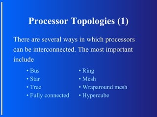
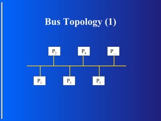
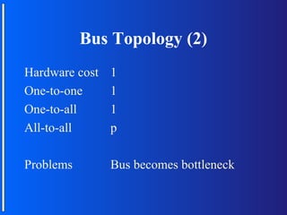
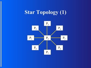
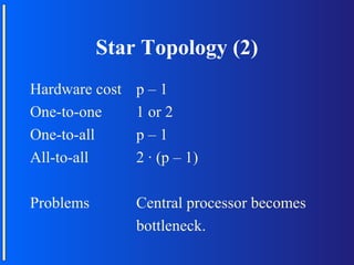
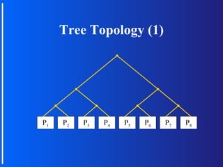
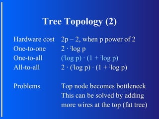
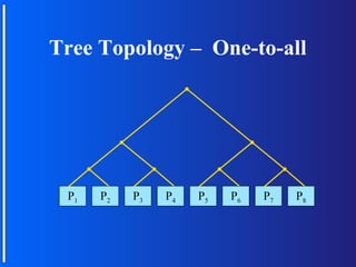
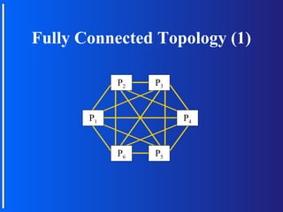
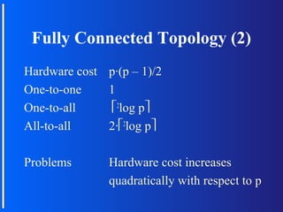
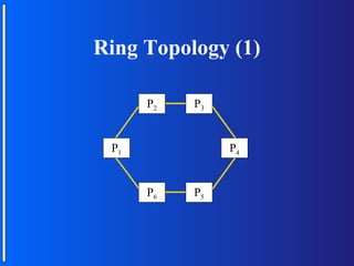
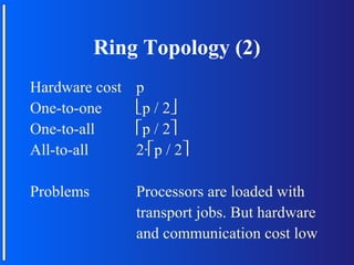
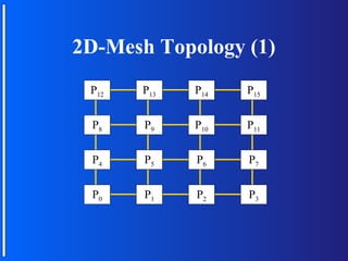
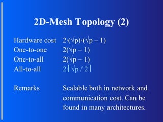
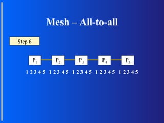
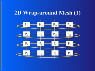
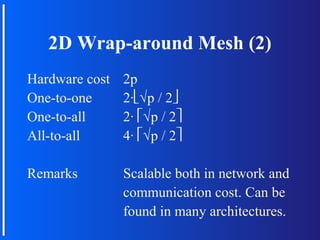
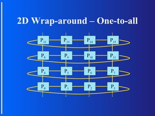
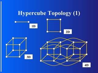
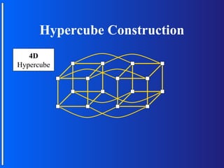
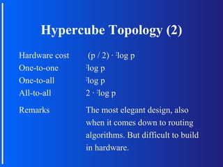
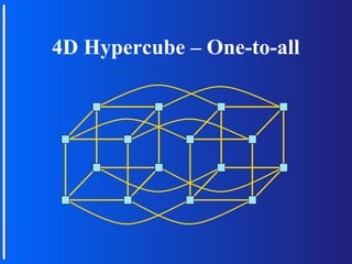
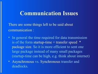
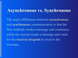
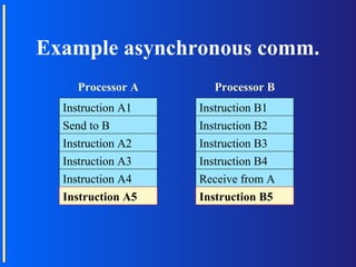
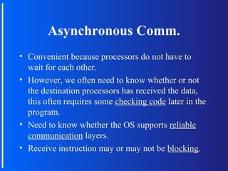
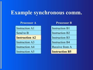
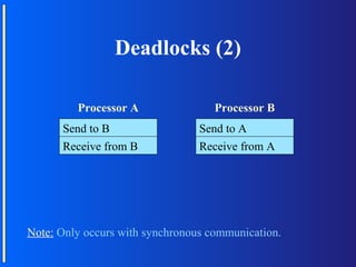
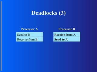
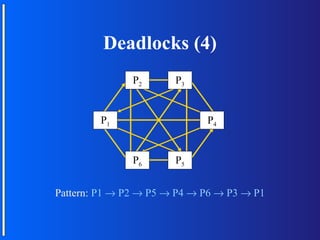
Introduction to Parallel
      Computing
         Part Ib
Processor Intercommunication
In part 1b we will look at the interconnection
network between processors. Using these
connections, various communication patterns
can be used to transport information from
one or more source processors, to one or more
destination processors.
Processor Topologies (1)
There are several ways in which processors
can be interconnected. The most important
include
    • Bus               • Ring
    • Star              • Mesh
    • Tree              • Wraparound mesh
    • Fully connected   • Hypercube
Topology Issues
Before looking at some of the major processor
topologies we have to know what makes a
certain topology well or ill suited to connect
processors.
There are two aspects of topologies that
should be looked at. These are scalability and
cost (communication and hardware).
Terminology
Communication is one-to-one when one
processor sends a message to another one.
In one-to-all or broadcast, one processor
  sends
a message to all other processors. In all-to-one
communication, all processors send their
message to one processor. Other forms of
communication include gather and all-to-all.
Connection Properties
There are three elements that are used in
Building the interconnection network. These
are the wire, a relay node, and a processor
node. The latter two elements can at a given
time send or receive only one message, no
matter how many wires enter or leave the
element.
Bus Topology (1)

      P2        P4        P…


P1         P3        P5
Bus Topology (2)
Hardware cost   1
One-to-one      1
One-to-all      1
All-to-all      p

Problems        Bus becomes bottleneck
Star Topology (1)
           P3
      P2        P4


 P1        P0        P5


      P8        P6
           P7
Star Topology (2)
Hardware cost   p–1
One-to-one      1 or 2
One-to-all      p–1
All-to-all      2 · (p – 1)

Problems        Central processor becomes
                bottleneck.
Tree Topology (1)


P1   P2   P3   P4   P5   P6   P7   P8
Tree Topology (2)
Hardware cost   2p – 2, when p power of 2
One-to-one      2 · 2log p
One-to-all      (2log p) · (1 + 2log p)
All-to-all      2 · (2log p) · (1 + 2log p)

Problems        Top node becomes bottleneck
                This can be solved by adding
                more wires at the top (fat tree)
Tree Topology – One-to-all


 P1   P2   P3   P4   P5   P6   P7   P8
Fully Connected Topology (1)

            P2   P3


       P1             P4


            P6   P5
Fully Connected Topology (2)
Hardware cost p·(p – 1)/2
One-to-one    1
One-to-all     2log p
All-to-all    2·2log p

Problems       Hardware cost increases
               quadratically with respect to p
Ring Topology (1)

      P2   P3


 P1             P4


      P6   P5
Ring Topology (2)
Hardware cost   p
One-to-one      p / 2
One-to-all      p / 2
All-to-all      2·p / 2

Problems        Processors are loaded with
                transport jobs. But hardware
                and communication cost low
2D-Mesh Topology (1)
 P12   P13   P14   P15


 P8    P9    P10   P11


 P4    P5    P6    P7


 P0    P1    P2    P3
2D-Mesh Topology (2)
Hardware cost   2·(√p)·(√p – 1)
One-to-one      2(√p – 1)
One-to-all      2(√p – 1)
All-to-all      2·√p / 2

Remarks         Scalable both in network and
                communication cost. Can be
                found in many architectures.
Mesh – All-to-all
Step 0
     6
     5
     4
     3
     2
     1


         P1     P2   P3      P4      P5

   1 23 45 1 23 45 1 23 45 1 23 45 1 23 45
2D Wrap-around Mesh (1)
   P12   P13   P14   P15


   P8    P9    P10   P11


   P4    P5    P6    P7


   P0    P1    P2    P3
2D Wrap-around Mesh (2)
Hardware cost   2p
One-to-one      2·√p / 2
One-to-all      2· √p / 2
All-to-all      4· √p / 2

Remarks         Scalable both in network and
                communication cost. Can be
                found in many architectures.
2D Wrap-around – One-to-all
     P12   P13   P14   P15


     P8    P9    P10   P11


     P4    P5    P6    P7


     P0    P1    P2    P3
Hypercube Topology (1)

        1D
                2D


   3D

                         4D
Hypercube Construction
   4D
   3D
   2D
   1D
Hypercube
Hypercube Topology (2)
Hardware cost     (p / 2) · 2log p
One-to-one      2
                 log p
One-to-all      2
                 log p
All-to-all      2 · 2log p
Remarks         The most elegant design, also
                when it comes down to routing
                algorithms. But difficult to build
                in hardware.
4D Hypercube – One-to-all
Communication Issues
There are some things left to be said about
communication :
• In general the time required for data transmission
  is of the form startup-time + transfer speed *
  package size. So it is more efficient to sent one
  large package instead of many small packages
  (startup-time can be high, e.g. think about internet)
• Asynchronous vs. Synchronous transfer and
  deadlocks.
Asynchronous vs. Synchronous
The major difference between asynchronous
and synchronous communication is that the
first methods sends a message and continues,
while the second sends a message and waits
for the receiver program to receive the
message.
Example asynchronous comm.
    Processor A      Processor B
  Instruction A1
  InstructionA1    Instruction B1
                   InstructionB1
  Send to B
  Send to B        Instruction B2
                   Instruction B2
  Instruction A2
  Instruction A2   Instruction B3
                   Instruction B3
  Instruction A3
  Instruction A3   Instruction B4
                   Instruction B4
  Instruction A4
  Instruction A4   Receive from A
                            from A
  Instruction A5
  Instruction A5   Instruction B5
                   Instruction B5
Asynchronous Comm.
• Convenient because processors do not have to
  wait for each other.
• However, we often need to know whether or not
  the destination processors has received the data,
  this often requires some checking code later in the
  program.
• Need to know whether the OS supports reliable
  communication layers.
• Receive instruction may or may not be blocking.
Example synchronous comm.
   Processor A      Processor B
 Instruction A1
 InstructionA1    Instruction B1
                  InstructionB1
 Send to B
 Send to B        Instruction B2
                  Instruction B2
 Instruction A2
 Instruction A2   Instruction B3
                  Instruction B3
 Instruction A3   Instruction B4
                  Instruction B4
 Instruction A4   Receive from A
                           from A
 Instruction A5   Instruction B5
                  Instruction B5
Synchronous comm.
• Both send and receive are blocking
• Processors have to wait for each other. This
  reduces efficiency.
• Implicitly offers a synchronisation point.
• Easy to program because fewer unexpected
  situations can arise.
• Problem: Deadlocks may occur.
Deadlocks (1)
A deadlock is a situation where two or more
processors are waiting to for each other
infinitely.
Deadlocks (2)

         Processor A                Processor B
      Send to B                  Send to A
      Receive from B             Receive from A


Note: Only occurs with synchronous communication.
Deadlocks (3)

  Processor A      Processor B
Send to B        Receive from A
Receive from B   Send to A
Deadlocks (4)
               P2      P3


        P1                   P4


               P6      P5


Pattern: P1 → P2 → P5 → P4 → P6 → P3 → P1
End of Part I
Are there any questions regarding part I

Parallel computing(1)

  • 1.
    Introduction to Parallel Computing Part Ib
  • 2.
    Processor Intercommunication In part1b we will look at the interconnection network between processors. Using these connections, various communication patterns can be used to transport information from one or more source processors, to one or more destination processors.
  • 3.
    Processor Topologies (1) Thereare several ways in which processors can be interconnected. The most important include • Bus • Ring • Star • Mesh • Tree • Wraparound mesh • Fully connected • Hypercube
  • 4.
    Topology Issues Before lookingat some of the major processor topologies we have to know what makes a certain topology well or ill suited to connect processors. There are two aspects of topologies that should be looked at. These are scalability and cost (communication and hardware).
  • 5.
    Terminology Communication is one-to-onewhen one processor sends a message to another one. In one-to-all or broadcast, one processor sends a message to all other processors. In all-to-one communication, all processors send their message to one processor. Other forms of communication include gather and all-to-all.
  • 6.
    Connection Properties There arethree elements that are used in Building the interconnection network. These are the wire, a relay node, and a processor node. The latter two elements can at a given time send or receive only one message, no matter how many wires enter or leave the element.
  • 7.
    Bus Topology (1) P2 P4 P… P1 P3 P5
  • 8.
    Bus Topology (2) Hardwarecost 1 One-to-one 1 One-to-all 1 All-to-all p Problems Bus becomes bottleneck
  • 9.
    Star Topology (1) P3 P2 P4 P1 P0 P5 P8 P6 P7
  • 10.
    Star Topology (2) Hardwarecost p–1 One-to-one 1 or 2 One-to-all p–1 All-to-all 2 · (p – 1) Problems Central processor becomes bottleneck.
  • 11.
    Tree Topology (1) P1 P2 P3 P4 P5 P6 P7 P8
  • 12.
    Tree Topology (2) Hardwarecost 2p – 2, when p power of 2 One-to-one 2 · 2log p One-to-all (2log p) · (1 + 2log p) All-to-all 2 · (2log p) · (1 + 2log p) Problems Top node becomes bottleneck This can be solved by adding more wires at the top (fat tree)
  • 13.
    Tree Topology –One-to-all P1 P2 P3 P4 P5 P6 P7 P8
  • 14.
    Fully Connected Topology(1) P2 P3 P1 P4 P6 P5
  • 15.
    Fully Connected Topology(2) Hardware cost p·(p – 1)/2 One-to-one 1 One-to-all 2log p All-to-all 2·2log p Problems Hardware cost increases quadratically with respect to p
  • 16.
    Ring Topology (1) P2 P3 P1 P4 P6 P5
  • 17.
    Ring Topology (2) Hardwarecost p One-to-one p / 2 One-to-all p / 2 All-to-all 2·p / 2 Problems Processors are loaded with transport jobs. But hardware and communication cost low
  • 18.
    2D-Mesh Topology (1) P12 P13 P14 P15 P8 P9 P10 P11 P4 P5 P6 P7 P0 P1 P2 P3
  • 19.
    2D-Mesh Topology (2) Hardwarecost 2·(√p)·(√p – 1) One-to-one 2(√p – 1) One-to-all 2(√p – 1) All-to-all 2·√p / 2 Remarks Scalable both in network and communication cost. Can be found in many architectures.
  • 20.
    Mesh – All-to-all Step0 6 5 4 3 2 1 P1 P2 P3 P4 P5 1 23 45 1 23 45 1 23 45 1 23 45 1 23 45
  • 21.
    2D Wrap-around Mesh(1) P12 P13 P14 P15 P8 P9 P10 P11 P4 P5 P6 P7 P0 P1 P2 P3
  • 22.
    2D Wrap-around Mesh(2) Hardware cost 2p One-to-one 2·√p / 2 One-to-all 2· √p / 2 All-to-all 4· √p / 2 Remarks Scalable both in network and communication cost. Can be found in many architectures.
  • 23.
    2D Wrap-around –One-to-all P12 P13 P14 P15 P8 P9 P10 P11 P4 P5 P6 P7 P0 P1 P2 P3
  • 24.
  • 25.
    Hypercube Construction 4D 3D 2D 1D Hypercube
  • 26.
    Hypercube Topology (2) Hardwarecost (p / 2) · 2log p One-to-one 2 log p One-to-all 2 log p All-to-all 2 · 2log p Remarks The most elegant design, also when it comes down to routing algorithms. But difficult to build in hardware.
  • 27.
    4D Hypercube –One-to-all
  • 28.
    Communication Issues There aresome things left to be said about communication : • In general the time required for data transmission is of the form startup-time + transfer speed * package size. So it is more efficient to sent one large package instead of many small packages (startup-time can be high, e.g. think about internet) • Asynchronous vs. Synchronous transfer and deadlocks.
  • 29.
    Asynchronous vs. Synchronous Themajor difference between asynchronous and synchronous communication is that the first methods sends a message and continues, while the second sends a message and waits for the receiver program to receive the message.
  • 30.
    Example asynchronous comm. Processor A Processor B Instruction A1 InstructionA1 Instruction B1 InstructionB1 Send to B Send to B Instruction B2 Instruction B2 Instruction A2 Instruction A2 Instruction B3 Instruction B3 Instruction A3 Instruction A3 Instruction B4 Instruction B4 Instruction A4 Instruction A4 Receive from A from A Instruction A5 Instruction A5 Instruction B5 Instruction B5
  • 31.
    Asynchronous Comm. • Convenientbecause processors do not have to wait for each other. • However, we often need to know whether or not the destination processors has received the data, this often requires some checking code later in the program. • Need to know whether the OS supports reliable communication layers. • Receive instruction may or may not be blocking.
  • 32.
    Example synchronous comm. Processor A Processor B Instruction A1 InstructionA1 Instruction B1 InstructionB1 Send to B Send to B Instruction B2 Instruction B2 Instruction A2 Instruction A2 Instruction B3 Instruction B3 Instruction A3 Instruction B4 Instruction B4 Instruction A4 Receive from A from A Instruction A5 Instruction B5 Instruction B5
  • 33.
    Synchronous comm. • Bothsend and receive are blocking • Processors have to wait for each other. This reduces efficiency. • Implicitly offers a synchronisation point. • Easy to program because fewer unexpected situations can arise. • Problem: Deadlocks may occur.
  • 34.
    Deadlocks (1) A deadlockis a situation where two or more processors are waiting to for each other infinitely.
  • 35.
    Deadlocks (2) Processor A Processor B Send to B Send to A Receive from B Receive from A Note: Only occurs with synchronous communication.
  • 36.
    Deadlocks (3) Processor A Processor B Send to B Receive from A Receive from B Send to A
  • 37.
    Deadlocks (4) P2 P3 P1 P4 P6 P5 Pattern: P1 → P2 → P5 → P4 → P6 → P3 → P1
  • 38.
    End of PartI Are there any questions regarding part I