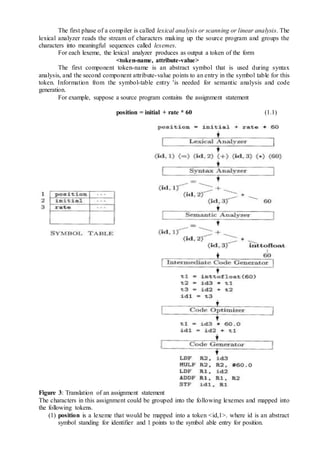
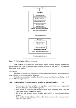
The document describes the various phases of a compiler: 1. Lexical analysis breaks the source code into tokens. 2. Syntax analysis generates a parse tree from the tokens. 3. Semantic analysis checks for semantic correctness using the parse tree and symbol table. 4. Intermediate code generation produces machine-independent code. 5. Code optimization improves the intermediate code. 6. Code generation translates the optimized code into target machine code.

1. Reg. No. :
B.E. / B.Tech. DEGREE EXAMINATION, MAY / JUNE 2016
Sixth Semester
Computer Science and Engineering
CS6660 – COMPILER DESIGN
(Regulation 2013)
Time : Three hours Maximum : 100 marks
Answer ALL Questions
Part A – (𝟏𝟎 × 𝟐 = 𝟐𝟎 marks)
1. What are the two parts of a Compilation? Explain briefly.
2. Illustrate diagrammatically how a language is processed.
3. Write a grammar for branching statements.
4. List the operations on languages.
5. Write the algorithm for FIRST and FOLLOW in parser.
6. Define ambiguous grammar.
7. What is DAG?
8. When does a Dangling reference occur?
9. What are the properties of optimizing Compiler?
10. Write the three address code sequence for the assignment statement
d:=(a-b)+(a-c)+(a-c).
Part B – (5 × 𝟏𝟔 = 𝟖𝟎 marks)
11 (a) Discus the various phases of compiler and trace it with the program statement
(position := initial + rate * 60).
(16)
Or
(b) (i) Explain language processing system with neat diagram. (8)
(ii) Explain the need for grouping of phases. (4)
(iii) Explain various Errors encountered in different phases of compiler. (4)
12 (a) (i) Differentiate between Lexeme, Tokens and pattern. (6)
(ii) What are the issues in lexical analysis? (4)
(iii) Write note on Regular Expressions. (6)
Or
(b) (i) Write notes on Regular expression to NFA. Construct Regular expression to NFA
for the sentence (a|b)*a.
(10)
(ii) Construct DFA to recognize the language (a/b)*ab (6)
13 (a) (i) Construct Stack implementation of shift reduce parsing for the grammar (8)
E → E + E
E → E * E
Question Paper Code : 57263

2. E → ( E )
E → id and the input string id1 + id2 * id3.
(ii) Explain LL(1) grammar for the sentence S → iEtS | iEtSeS | a E → b. (8)
Or
(b) (i) Write an algorithm for Non Recursive Predictive Parser. (6)
(ii) Explain Context free grammar with examples. (10)
14 (a) (i) Construct a syntax directed definitions for constructing a syntax tree for
assignment statements. (8)
S → id := E
E → E1 + E2
E → E1 * E2
E → - E1
E → ( E1 )
E → id
(ii) Discuss specification of a simple type checker. (8)
Or
(b) Discuss different storage allocation strategies. (16)
15 (a) Explain Principal sources of optimization with examples. (16)
Or
(b) (i) Explain various issues in the design of code generator. (8)
(ii) Write note on Simple code generator. (8)
All the Best – No substitute for hard work.
Mr. G. Appasami SET,NET,GATE,M.Sc., M.C.A., M.Phil., M.Tech., (P.hd.), MISTE,MIETE,AMIE, MCSI, MIAE, MIACSIT, MASCAP,
MIARCS, MISIAM, MISCE, MIMS, MISCA, MISAET, PGDTS, PGDBA, PGDHN,PGDST,(AP / CSE / DRPEC).

3. ANSWER KEY
B.E. / B.Tech. DEGREE EXAMINATION, MAY / JUNE 2016
Sixth Semester
Computer Science and Engineering
CS6660 – COMPILER DESIGN
(Regulation 2013)
Time : Three hours Maximum : 100 marks
Answer ALL Questions
Part A – (𝟏𝟎 × 𝟐 = 𝟐𝟎 marks)
1. What are the two parts of a Compilation? Explain briefly.
The process of compilation carried out in two parts, they are analysis and synthesis. The
analysis part breaks up the source program into constituent pieces and imposes a grammatical
structure on them.
The analysis part carried out in three phases, they are lexical analysis, syntax analysis
and Semantic Analysis. The analysis part is often called the front end of the compiler.
The synthesis part constructs the desired target program from the intermediate
representation and the information in the symbol table.
The synthesis part carried out in three phases, they are Intermediate Code Generation,
Code Optimization and Code Generation. The synthesis part is called the back end of the
compiler.
2. Illustrate diagrammatically how a language is processed.
Figure 1: A language-processing system
3. Write a grammar for branching statements.
Statement  if Expression then Statement | if Expression then Statement else Statement | a ;
Expression  b
i.e., S  i E t S | i E t S e S | a ;
E  b
Grammar G = (V, T, P, S) = ({S, E}, {i, t, e, a, b}, { S  i E t S | i E t S e S | a ; E  b}, S )

4. 4. List the operations on languages.
Example: Let L be the set of letters {A, B, . . . , Z, a, b, . . . , z) and let D be the set of digits
{0,1,.. .9). Other languages that can be constructed from languages L and D
1. L U D is the set of letters and digits - strictly speaking the language with 62 strings of
length one, each of which strings is either one letter or one digit.
2. LD is the set df 520 strings of length two, each consisting of one letter followed by
one digit.
3. L4 is the set of all 4-letter strings.
4. L* is the set of ail strings of letters, including e, the empty string.
5. L(L U D)* is the set of all strings of letters and digits beginning with a letter.
6. D+ is the set of all strings of one or more digits.
5. Write the algorithm for FIRST and FOLLOW in parser.
To compute FIRST(X) for all grammar symbols X, apply the following rules until no more
terminals or E: can be added to any FIRST set.
1. If X is a terminal, then FIRST(X) = {X}.
2. If X is a nonterminal and X  YlY2…Yk is a production for some k≥1, then place a in
FIRST(X) if for some i, a is in FIRST(Yi), and ε is in all of FIRST(Y1),…, FIRST(Yi-1);
that is, Yl… Yi-1 =>* ε. (If ε is in FIRST(Yj) for all j = 1,2, . . . , k, then add ε to
FIRST(X). For example, everything in FIRST(Yl) is surely in FIRST(X). If Yl does not
derive ε, then we add nothing more to FIRST(X), but if Yl =>* ε, then we add
F1RST(Y2), and So on.)
3. If X ε is a production, then add ε to FIRST(X).
To compute FOLLOW(A) for all nonterminals A, apply the following rules until nothing can be
added to any FOLLOW set.
1. Place $ in FOLLOW(S), where S is the start symbol, and $ is the input right endmarker.
2. If there is a production AαBβ, then everything in FIRST(β) except ε is in
FOLLOW(B).
3. If there is a production AαB, or a production AαBβ, where FIRST(β) contains ε, then
everything in FOLLOW (A) is in FOLLOW (B).
6. Define ambiguous grammar.
A grammar that produces more than one parse tree for some sentence is said to be
ambiguous.
A grammar G is said to be ambiguous if it has more than one parse tree either in LMD or
in RMD for at least one string.
Example: E  E + E | E * E | id
7. What is DAG?
Directed Acyclic Graph (DAG) is a tool that depicts the structure of basic blocks, helps to
see the flow of values flowing among the basic blocks, and offers optimization too. DAG
provides easy transformation on basic blocks. DAG can be understood here:
 Leaf nodes represent identifiers, names or constants.
 Interior nodes represent operators.
 Interior nodes also represent the results of expressions or the identifiers/name where the
values are to be stored or assigned.

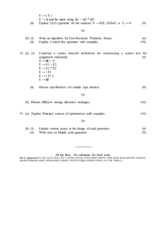
5. 8. When does a Dangling reference occur?
1. A dangling reference occurs when there is a reference to storage that has been
deallocated.
2. It is a logical error to use dangling references, Since the value of deallocated storage
is undefined according to the semantics of most languages.
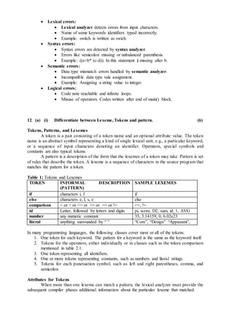
9. What are the properties of optimizing Compiler?
THE PRINCIPAL SOURCES OF OPTIMIZATION
Semantics Preserving Transformations (Functions ) - Safeguards original program
meaning
Global Common Subexpressions
Copy Propagation
Dead-Code Elimination
Code Motion / Movement
Induction Variables and Reduction in Strength
OPTIMIZATION OF BASIC BLOCKS
The DAG Representation of Basic Blocks
Finding Local Common Subexpressions
Dead Code Elimination
The Use of Algebraic Identities
Representation of Array References
Pointer Assignments and Procedure Calls
Reassembling Basic Blocks from DAG's
PEEPHOLE OPTIMIZATION
Eliminating Redundant Loads and Stores
Eliminating Unreachable Code
Flow-of-Control Optimizations
Algebraic Simplification and Reduction in Strength
Use of Machine Idioms
LOOP OPTINIZATION
Code Motion while(i<max-1) {sum=sum+a[i]}
=> n= max-1; while(i<n) {sum=sum+a[i]}
Induction Variables and Strength Reduction: only 1 Induction Variable in loop, either
i++ or j=j+2, * by +
Loop invariant method
Loop unrolling
Loop fusion
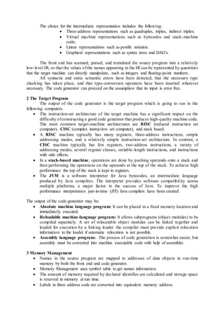
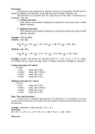
10. Write the three address code sequence for the assignment statement
d:=(a-b)+(a-c)+(a-c).
Three address code sequence
t1=a-b
t2=a-c
t3=t1+t2
t4=t3+t2
d=t4

6. Part B – (5 × 𝟏𝟔 = 𝟖𝟎 marks)
11 (a) Discus the various phases of compiler and trace it with the program statement
(position := initial + rate * 60). (16)
The process of compilation carried out in two parts, they are analysis and synthesis. The
analysis part breaks up the source program into constituent pieces and imposes a grammatical
structure on them.
It then uses this structure to create an intermediate representation of the source program.
The analysis part also collects information about the source program and stores it in a data
structure called a symbol table, which is passed along with the intermediate representation to the
synthesis part.
The analysis part carried out in three phases, they are lexical analysis, syntax analysis
and Semantic Analysis. The analysis part is often called the front end of the compiler. The
synthesis part constructs the desired target program from the intermediate representation and the
information in the symbol table.
The synthesis part carried out in three phases, they are Intermediate Code Generation,
Code Optimization and Code Generation. The synthesis part is called the back end of the
compiler.
Figure 2: Phases of a compiler
11.1 Lexical Analysis

7. The first phase of a compiler is called lexical analysis or scanning or linear analysis. The
lexical analyzer reads the stream of characters making up the source program and groups the
characters into meaningful sequences called lexemes.
For each lexeme, the lexical analyzer produces as output a token of the form
<token-name, attribute-value>
The first component token-name is an abstract symbol that is used during syntax
analysis, and the second component attribute-value points to an entry in the symbol table for this
token. Information from the symbol-table entry 'is needed for semantic analysis and code
generation.
For example, suppose a source program contains the assignment statement
position = initial + rate * 60 (1.1)
Figure 3: Translation of an assignment statement
The characters in this assignment could be grouped into the following lexemes and mapped into
the following tokens.
(1) position is a lexeme that would be mapped into a token <id,1>. where id is an abstract
symbol standing for identifier and 1 points to the symbol able entry for position.

8. (2) The assignment symbol = is a lexeme that is mapped into the token <=>.
(3) initial is a lexeme that is mapped into the token <id, 2>.
(4) + is a lexeme that is mapped into the token <+>.
(5) rate is a lexeme that is mapped into the token <id, 3>.
(6) * is a lexeme that is mapped into the token <*>.
(7) 60 is a lexeme that is mapped into the token <60>.
Blanks separating the lexemes would be discarded by the lexical analyzer. The sequence of
tokens produced as follows after lexical analysis.
<id, 1> <=> <id, 2> <+> <id, 3> <*> <60> (1.2)
11.2 Syntax Analysis
The second phase of the compiler is syntax analysis or parsing or hierarchical analysis.
The parser uses the first components of the tokens produced by the lexical analyzer to
create a tree-like intermediate representation that depicts the grammatical structure of the token
stream.
The hierarchical tree structure generated in this phase is called parse tree or syntax tree.
In a syntax tree, each interior node represents an operation and the children of the node
represent the arguments of the operation.
Figure 4: Syntax tree for position = initial + rate * 60
The tree has an interior node labeled * with <id, 3> as its left child and the integer 60 as
its right child. The node <id, 3> represents the identifier rate. Similarly <id,2> and <id, 1> are
represented as in tree. The root of the tree, labeled =, indicates that we must store the result of
this addition into the location for the identifier position.
11.3 Semantic Analysis
The semantic analyzer uses the syntax tree and the information in the symbol table to
check the source program for semantic consistency with the language definition.
It ensures the correctness of the program, matching of the parenthesis is also done in this
phase.
It also gathers type information and saves it in either the syntax tree or the symbol table,
for subsequent use during intermediate-code generation.
An important part of semantic analysis is type checking, where the compiler checks that
each operator has matching operands.
The compiler must report an error if a floating-point number is used to index an array.
The language specification may permit some type conversions like integer to float for float
addition is called coercions.
The operator * is applied to a floating-point number rate and an integer 60. The integer
may be converted into a floating-point number by the operator inttofloat explicitly as shown in
the figure.
Figure 5: Semantic tree for position = initial + rate * 60
11.4 Intermediate Code Generation
After syntax and semantic analysis of the source program, many compilers generate an
explicit low-level or machine-like intermediate representation.

9. The intermediate representation have two important properties:
a. It should be easy to produce
b. It should be easy to translate into the target machine.
Three-address code is one of the intermediate representations, which consists of a
sequence of assembly-like instructions with three operands per instruction. Each operand can act
like a register.
The output of the intermediate code generator in Figure 1.8 consists of the three-address code
sequence for position = initial + rate * 60
t1 = inttofloat(60)
t2 = id3 * t1
t3 = id2 + t2
id1 = t3 (1.3)
11.5 Code Optimization
The machine-independent code-optimization phase attempts to improve the intermediate
code so that better target code will result. Usually better means faster.
Optimization has to improve the efficiency of code so that the target program running
time and consumption of memory can be reduced.
The optimizer can deduce that the conversion of 60 from integer to floating point can be
done once and for all at compile time, so the inttofloat operation can be eliminated by replacing
the integer 60 by the floating-point number 60.0.
Moreover, t3 is used only once to transmit its value to id1 so the optimizer can transform
(1.3) into the shorter sequence
t1 = id3 * 60.0
id1 = id2 + t1 (1.4)
11.6 Code Generation
The code generator takes as input an intermediate representation of the source program
and maps it into the target language.
If the target language is machine code, then the registers or memory locations are
selected for each of the variables used by the program.
The intermediate instructions are translated into sequences of machine instructions.
For example, using registers R1 and R2, the intermediate code in (1.4) might get
translated into the machine code
LDF R2, id3
MULF R2, R2 , #60.0
LDF Rl, id2
ADDF Rl, Rl, R2
STF idl, Rl (1.5)
The first operand of each instruction specifies a destination. The F in each instruction
tells us that it deals with floating-point numbers.
The code in (1.5) loads the contents of address id3 into register R2, then multiplies it
with floating-point constant 60.0. The # signifies that 60.0 is to be treated as an immediate
constant. The third instruction moves id2 into register R1 and the fourth adds to it the value
previously computed in register R2. Finally, the value in register R1 is stored into the address of
id1, so the code correctly implements the assignment statement (1.1).
Or
11 (b) (i) Explain language processing systemwith neat diagram. (8)
In addition to a compiler, several other programs may be required to create an executable
target program, as shown in Figure 6.

10. Preprocessor: Preprocessor collects the source program which is divided into modules and
stored in separate files. The preprocessor may also expand shorthands called macros into source
language statements. E.g. # include<math.h>, #define PI .14
Compiler: The modified source program is then fed to a compiler. The compiler may produce
an assembly-language program as its output. because assembly language is easier to produce as
output and is easier to debug.
Assembler: The assembly language is then processed by a program called an assembler that
produces relocatable machine code as its output.
Linker: The linker resolves external memory addresses, where the code in one file may refer to
a location in another file. Large programs are often compiled in pieces, so the relocatable
machine code may have to be linked together with other relocatable object files and library files
into the code that actually runs on the machine.
Loader: The loader then puts together all of the executable object files into memory for
execution. It also performs relocation of an object code.
Figure 6: A language-processing system
Note: Preprocessors, Assemblers, Linkers and Loader are collectively called cousins of
compiler.
(ii) Explain the need for grouping of phases. (4)
 Each phases deals with the logical organization of a compiler.
 Activities of several phases may be grouped together into a pass that reads an
input file and writes an output file.
 The front-end phases of lexical analysis, syntax analysis, semantic analysis, and
intermediate code generation might be grouped together into one pass.
 Code optimization might be an optional pass.
 A back end pass consisting of code generation for a particular target machine.

11. Figure 7: The Grouping of Phases of compiler
Some compiler collections have been created around carefully designed intermediate
representations that allow the front end for a particular language to interface with the back end
for a certain target machine.
Advantages:
With these collections, we can produce compilers for different source languages for one
target machine by combining different front ends.
Similarly, we can produce compilers for different target machines, by combining a front
end for different target machines.
(iii) Explain various Errors encountered in different phases of compiler. (4)
 An important role of the compiler is to report any errors in the source program that
it detects during the entire translation process.
 Each phases of compiler can encounter errors, after detecting errors, must be
corrected to precede compilation process.
 The syntax and semantic phases handles large number of errors in compilation
process.
 Error handler handles all types of errors like lexical errors, syntax errors, semantic
errors and logical errors.
Front end
Source language dependent
(Machine independent)
Lexical Analyzer
Syntax analyzer
SemanticAnalyzer
Intermediate
Code Generator
Source program (input)
Target program (output)
Back end
Machine dependent
(Source language dependent)
Code optimizer
(optional)
Code Generator
Intermediate code

12.  Lexical errors:
 Lexical analyzer detects errors from input characters.
 Name of some keywords identifiers typed incorrectly.
 Example: switch is written as swich.
 Syntax errors:
 Syntax errors are detected by syntax analyzer.
 Errors like semicolon missing or unbalanced parenthesis.
 Example: ((a+b* (c-d)). In this statement ) missing after b.
 Semantic errors:
 Data type mismatch errors handled by semantic analyzer.
 Incompatible data type vale assignment.
 Example: Assigning a string value to integer.
 Logical errors:
 Code note reachable and infinite loops.
 Misuse of operators. Codes written after end of main() block.
12 (a) (i) Differentiate between Lexeme, Tokens and pattern. (6)
Tokens, Patterns, and Lexemes
A token is a pair consisting of a token name and an optional attribute value. The token
name is an abstract symbol representing a kind of single lexical unit, e.g., a particular keyword,
or a sequence of input characters denoting an identifier. Operators, special symbols and
constants are also typical tokens.
A pattern is a description of the form that the lexemes of a token may take. Pattern is set
of rules that describe the token. A lexeme is a sequence of characters in the source program that
matches the pattern for a token.
Table 1: Tokens and Lexemes
TOKEN INFORMAL DESCRIPTION
(PATTERN)
SAMPLE LEXEMES
if characters i, f if
else characters e, l, s, e else
comparison < or > or <= or >= or == or != <=, !=
id Letter, followed by letters and digits pi, score, D2, sum, id_1, AVG
number any numeric constant 35, 3.14159, 0, 6.02e23
literal anything surrounded by “ ” “Core”, “Design” “Appasami”,
In many programming languages, the following classes cover most or all of the tokens:
1. One token for each keyword. The pattern for a keyword is the same as the keyword itself.
2. Tokens for the operators, either individually or in classes such as the token comparison
mentioned in table 2.1.
3. One token representing all identifiers.
4. One or more tokens representing constants, such as numbers and literal strings.
5. Tokens for each punctuation symbol, such as left and right parentheses, comma, and
semicolon
Attributes for Tokens
When more than one lexeme can match a pattern, the lexical analyzer must provide the
subsequent compiler phases additional information about the particular lexeme that matched.

13. The lexical analyzer returns to the parser not only a token name, but an attribute value
that describes the lexeme represented by the token.
The token name influences parsing decisions, while the attribute value influences
translation of tokens after the parse.
Information about an identifier - e.g., its lexeme, its type, and the location at which it is
first found (in case an error message) - is kept in the symbol table.
Thus, the appropriate attribute value for an identifier is a pointer to the symbol-table
entry for that identifier.
Example: The token names and associated attribute values for the Fortran statement
E = M * C ** 2 are written below as a sequence of pairs.
<id, pointer to symbol-table entry for E>
< assign_op >
<id, pointer to symbol-table entry for M>
<mult_op>
<id, pointer to symbol-table entry for C>
<exp_op>
<number, integer value 2 >
Note that in certain pairs, especially operators, punctuation, and keywords, there is no
need for an attribute value. In this example, the token number has been given an integer-valued
attribute.
(ii) What are the issues in lexical analysis? (4)
1. Simplicity of design: It is the most important consideration. The separation of lexical
and syntactic analysis often allows us to simplify tasks. whitespace and comments
removed by the lexical analyzer.
2. Compiler efficiency is improved. A separate lexical analyzer allows us to apply
specialized techniques that serve only the lexical task, not the job of parsing. In addition,
specialized buffering techniques for reading input characters can speed up the compiler
significantly.
3. Compiler portability is enhanced. Input-device-specific peculiarities can be restricted
to the lexical analyzer.
(iii) Write note on Regular Expressions. (6)
Regular expression can be defined as a sequence of symbols and characters expressing a
string or pattern to be searched.
Regular expressions are mathematical representation which describes the set of strings of
specific language.
Regular expression for identifiers represented by letter_ ( letter_ | digit )*. The vertical
bar means union, the parentheses are used to group subexpressions, and the star means "zero or
more occurrences of".
Each regular expression r denotes a language L(r), which is also defined recursively from
the languages denoted by r's subexpressions.
The rules that define the regular expressions over some alphabet Σ.
Basis rules:
1. ε is a regular expression, and L(ε) is { ε }.
2. If a is a symbol in Σ , then a is a regular expression, and L(a) = {a}, that is,
the language with one string of length one.

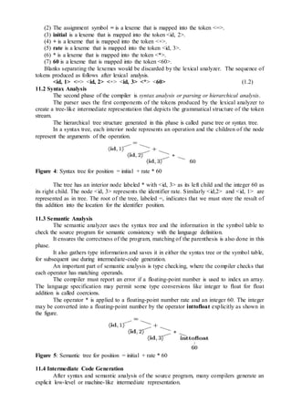
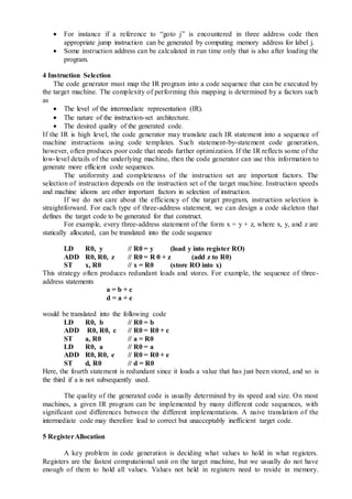
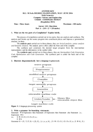
14. Induction rules: Suppose r and s are regular expressions denoting languages L(r) and L(s),
respectively.
1. (r) | (s) is a regular expression denoting the language L(r) U L(s).
2. (r) (s) is a regular expression denoting the language L(r) L(s) .
3. (r) * is a regular expression denoting (L (r)) * .
4. (r) is a regular expression denoting L(r). i.e., Additional pairs of parentheses
around expressions.
Example: Let Σ = {a, b}.
Regular
expression
Language Meaning
a|b {a, b} Single ‘a’ or ‘b’
(a|b) (a|b) {aa, ab, ba, bb} All strings of length two over the alphabet Σ
a* { ε, a, aa, aaa, …} Consisting of all strings of zero or more a's
(a|b)* {ε, a, b, aa, ab, ba, bb,
aaa, …}
set of all strings consisting of zero or more
instances of a or b
a|a*b {a, b, ab, aab, aaab, …} String a and all strings consisting of zero or
more a's and ending in b
A language that can be defined by a regular expression is called a regular set. If two
regular expressions r and s denote the same regular set, we say they are equivalent and write r =
s. For instance, (a|b) = (b|a), (a|b)*= (a*b*)*, (b|a)*= (a|b)*, (a|b) (b|a) =aa|ab|ba|bb.
Extensions of Regular Expressions
Few notational extensions that were first incorporated into Unix utilities such as Lex that
are particularly useful in the specification lexical analyzers.
1. One or more instances: The unary, postfix operator + represents the positive closure
of a regular expression and its language. If r is a regular expression, then (r)+ denotes
the language (L(r))+. The two useful algebraic laws, r* = r+|ε and r+ = rr* = r*r.
2. Zero or one instance: The unary postfix operator ? means "zero or one occurrence."
That is, r? is equivalent to r|ε , L(r?) = L(r) U {ε}.
3. Character classes: A regular expression a1|a2|…|an, where the ai's are each symbols
of the alphabet, can be replaced by the shorthand [a1, a2, …an]. Thus, [abc] is
shorthand for a|b|c, and [a-z] is shorthand for a|b|…|z.
Example: Regular definition for C identifier
Letter_  [A-Z a-z_]
digit  [0-9]
id letter_ ( letter_ | digit )*
Example: Regular definition unsigned integer
digit  [0-9]
digits  digit+
number  digits ( . digits)? ( E [+ -]? digits )?
Note: The operators *, +, and ? has the same precedence and associativity.
Or

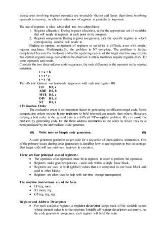
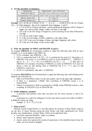
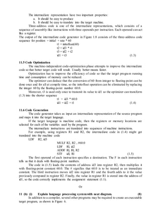
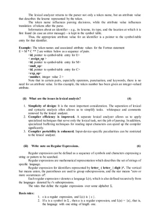
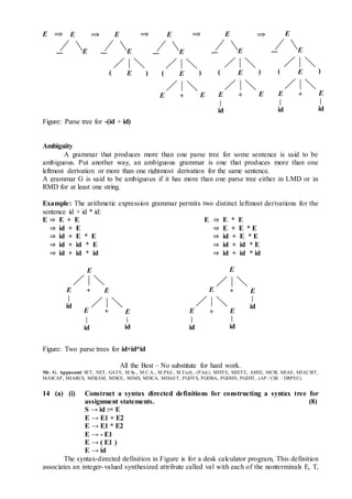
15. 12 (b) (i) Write notes on Regular expression to NFA. Construct Regular expression to
NFA for the sentence (a|b)*a. (10)
Consider the regular expression r = (a|b)*a
Augmented regular expression r = (a|b)*◦a◦#
1 2 3 4
Syntax tree for (a|b)*a#
firstpos and lastpos for nodes in the syntax tree for (a|b)*a#
NODE n Followpos(n)
1 {1, 2, 3}
2 {1, 2, 3}
3 {4}
4 { }
The value of firstpos for the root of the tree is {1,2,3}, so this set is the start state of D.
all this set of states A. We must compute Dtran[A, a] and Dtran[A, b]. Among the positions of
A, 1 and 3 correspond to a, while 2 corresponds to b. Thus, Dtran[A, a] = followpos(1) U
followpos(3) = {1, 2,3,4}, and Dtran[A, b] = followpos(2) = {1,2,3}.
123 1234
b
a
b a
{2} b {2}
{1, 2} | {1,2}
{1} a {1}
{1,2,3}◦ {3}
{1, 2} * {1, 2} {3} a {3}
{4} # {4}
{1,2,3}◦ {4}
b
2
|
* a
3
a
1
◦ #
4
◦

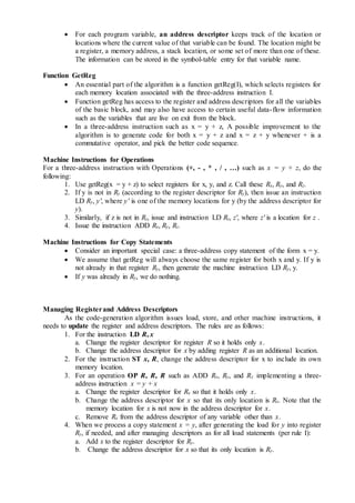
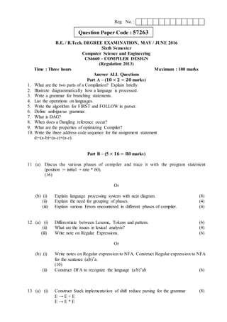
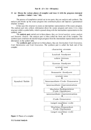
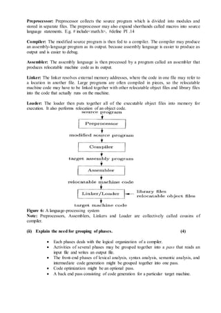
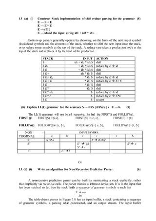
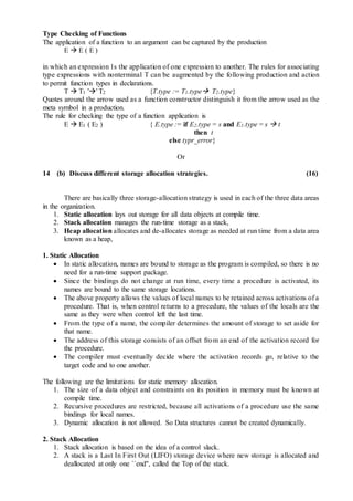
16. (ii) Construct DFA to recognize the language (a/b)*ab (6)
Consider the regular expression r = (a|b)*ab
Augmented regular expression r = (a|b)*◦a◦b◦#
1 2 3 4 5
Syntax tree for (a|b)*a#
firstpos and lastpos for nodes in the syntax tree for (a|b)*ab#
NODE n Followpos(n)
1 {1, 2, 3}
2 {1, 2, 3}
3 {4}
4 {5 }
5 { }
The value of firstpos for the root of the tree is {1,2,3}, so this set is the start state of D.
all this set of states A. We must compute Dtran[A, a] and Dtran[A, b]. Among the positions of
A, 1 and 3 correspond to a, while 2 corresponds to b. Thus, Dtran[A, a] = followpos(1) U
followpos(3) = {1, 2,3,4}, and Dtran[A, b] = followpos(2) = {1,2,3}.
123
b
a
b a
12351234
b
a
{2} b {2}
{1, 2} | {1,2}
{1} a {1}
{1,2,3}◦ {3}
{1, 2} * {1, 2} {3} a {3}
{4} b {4}
{1,2,3}◦ {4} {5} # {5}
{1,2,3}◦ {5}
b
2
|
* a
3
a
1
◦ b
4
◦ #
5
◦

17. 13 (a) (i) Construct Stack implementation of shift reduce parsing for the grammar (8)
E → E + E
E → E * E
E → ( E )
E → idand the input string id1 + id2 * id3.
Bottom-up parsers generally operate by choosing, on the basis of the next input symbol
(lookahead symbol) and the contents of the stack, whether to shift the next input onto the stack,
or to reduce some symbols at the top of the stack. A reduce step takes a production body at the
top of the stack and replaces it by the head of the production.
STACK INPUT ACTION
$ id1 + id2 * id3 $ shift
$ id1 + id2 * id3 $ reduce by E  id
$ E + id2 * id3 $ shift
$ E+ id2 * id3 $ shift
$ E+ id2 * id3 $ reduce by E  id
$ E+ E * id3 $ reduce by E  E+E
$ E * id3 $ shift
$ E* id3 $ shift
$ E* id3 $ reduce by E  id
$ E* E $ reduce by E  E*E
$ E $ accept
(ii) Explain LL(1) grammar for the sentence S → iEtS | iEtSeS | a E → b. (8)
The LL(1) grammar will not be left recursive. So find the FIRST() and FOLLOW().
FIRST (): FIRST(S) ={i,a}, FIRST(S') ={e, ε}, FIRST(E) ={b}
FOLLOW(): FOLLOW(S)={e, $}, FOLLOW(S')={ e, $}, FOLLOW(E)={t, $}
NON -
TERMINAL
INPUT SYMBOL
a b e i t $
S S  a S  iEtSS'
S' S'  eS
S'  ε
S'  ε
E E  b
Or
13 (b) (i) Write an algorithm for Non Recursive Predictive Parser. (6)
A nonrecursive predictive parser can be built by maintaining a stack explicitly, rather
than implicitly via recursive calls. The parser mimics a leftmost derivation. If w is the input that
has been matched so far, then the stack holds a sequence of grammar symbols α such that
S
∗
⇒ wa
lm
The table-driven parser in Figure 3.8 has an input buffer, a stack containing a sequence
of grammar symbols, a parsing table constructed, and an output stream. The input buffer

18. contains the string to be parsed, followed by the endmarker $. We reuse the symbol $ to mark
the bottom of the stack, which initially contains the start symbol of the grammar on top of $.
The parser is controlled by a program that considers X, the symbol on top of the stack,
and a, the current input symbol. If X is a nonterminal, the parser chooses an X-production by
consulting entry M[X, a] of the parsing table M. Otherwise, it checks for a match between the
terminal X and current input symbol a.
Figure: Model of a table-driven predictive parser
Algorithm 3.3 : Table-driven predictive parsing.
INPUT: A string w and a parsing table M for grammar G.
OUTPUT: If w is in L(G), a leftmost derivation of w; otherwise, an error indication.
METHOD: Initially, the parser is in a configuration with w$ in the input buffer and the start
symbol S of G on top of the stack, above $. The following procedure uses the predictive parsing
table M to produce a predictive parse for the input.
set ip to point to the first symbol of w;
set X to the top stack symbol;
while ( X ≠ $ ) { /* stack is not empty */
if ( X is a ) pop the stack and advance ip;
else if ( X is a terminal ) error();
else if ( M[X, a] is an error entry ) error();
else if ( M[X,a] = X  Y1Y2…Yk) {
output the production X  Y1Y2…Yk;
pop the stack;
push YkYk-1…Y1 onto the stack, with Yl on top;
}
set X to the top stack symbol;
}
(ii) Explain Context free grammar with examples. (10)
The Formal Definition of a Context-Free Grammar
A context-free grammar G is defined by the 4-tuple: G= (V, T, P S) where
1. V is a finite set of non-terminals (variable).
2. T is a finite set of terminals.
3. P is a finite set of production rules of the form Aα. Where A is nonterminal
and α is string of terminals and/or nonterminals. P is a relation
from V to (V∪T)*.
4. S is the start symbol (variable S∈V).
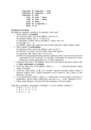
Example : The following grammar defines simple arithmetic expressions. In this grammar, the
terminal symbols are id + - * / ( ). The nonterminal symbols are expression, term and factor, and
expression is the start symbol.
Input
Stack
Predictive
Parsing
Program
Parsing
Table M
OutputX
Y
Z
$
a + b $

19. expression  expression + term
expression  expression - term
expression  term
term  term * factor
term  term / factor
term  factor
factor  ( expression )
factor  id
Notational Conventions
The following notational conventions for grammars can be used
1. These symbols are terminals:
(a) Lowercase letters early in the alphabet, such as a, b, e.
(b) Operator symbols such as +,*, and so on.
(c) Punctuation symbols such as parentheses, comma, and so on.
(d) The digits 0,1,. . . ,9.
(e) Boldface strings such as id or if, each of which represents a single terminal symbol.
2. These symbols are nonterminals:
(a) Uppercase letters early in the alphabet, such as A, B, C.
(b) The letter S is usually the start symbol when which appears.
(c) Lowercase, italic names such as expr or stmt.
(d) When discussing programming constructs, uppercase letters may be used to represent
nonterminals for the constructs. For example, nonterminals for expressions, terms,
and factors are often represented by E, T, and F, respectively.
3. Uppercase letters late in the alphabet, such as X, Y, Z, represent grammar symbols; that
is, either nonterminals or terminals.
4. Lowercase letters late in the alphabet, chiefly u, v, . . . , z, represent (possibly empty)
strings of terminals.
5. Lowercase Greek letters, α, β, γ for example, represent (possibly empty) strings of
grammar symbols. Thus, a generic production can be written as A α, where A is the
head and α the body.
6. A set of productions A α1 , A α2 ,…, A αk with a common head A (call them A-
productions), may be written A α1 | α2 |…| αk. call α1, α2,…, αk the Alternatives for A.
7. Unless stated otherwise, the head of the first production is the start symbol.
Using these conventions, the grammar of Example 3.1 can be rewritten concisely as
E  E + T | E - T | T
T  T * F | T / F | F
F  ( E ) | id

20. Derivations
The derivation uses productions to generate a string (set of terminals). The derivation is
formed by replacing the nonterminal in the right hand side by suitable production rule.
The derivations are classified into two types based on the order of replacement of
production. They are:
1. Leftmost derivation
If the leftmost non-terminal is replaced by its production in derivation, then it called
leftmost derivation.
2. Rightmost derivation
If the rightmost non-terminal is replaced by its production in derivation, then it called
rightmost derivation.
Example: LMD and RMD
LMD for - ( id + id )
E
𝒍𝒎
⇒ - E
𝒍𝒎
⇒ - ( E )
𝒍𝒎
⇒ - ( E + E )
𝒍𝒎
⇒ - ( id + E )
𝒍𝒎
⇒ - ( id + id )
RMD for - ( id + id )
E
𝒓𝒎
⇒ - E
𝒓𝒎
⇒ - ( E )
𝒓𝒎
⇒ - ( E + E )
𝒓𝒎
⇒ - ( E + id )
𝒓𝒎
⇒ - ( id + id )
Example: Consider the context free grammar (CFG) G = ({S}, {a, b, c}, P, S ) where
P={SSbS | ScS | a}. Derive the string “abaca” by leftmost derivation and rightmost derivation.
Leftmost derivation for “abaca”
S ⇒ SbS
⇒ abS (using rule S  a)
⇒ abScS (using rule S  ScS )
⇒ abacS (using rule S  a)
⇒ abaca (using rule S  a)
Rightmost derivation for “abaca”
S ⇒ ScS
⇒ Sca (using rule S  a)
⇒ SbSca (using rule S  SbS )
⇒ Sbaca (using rule S  a)
⇒ abaca (using rule S  a)
Parse Trees and Derivations
A parse tree is a graphical representation of a derivation. t is convenient to see how
strings are derived from the start symbol. The start symbol of the derivation becomes the root of
the parse tree.
Example: construction of parse tree for - ( id + id )
Derivation:
E ⇒ - E ⇒ - ( E ) ⇒ - ( E + E ) ⇒ - ( id + E ) ⇒ - ( id + id )
Parse tree:

21. Figure: Parse tree for -(id + id)
Ambiguity
A grammar that produces more than one parse tree for some sentence is said to be
ambiguous. Put another way, an ambiguous grammar is one that produces more than one
leftmost derivation or more than one rightmost derivation for the same sentence.
A grammar G is said to be ambiguous if it has more than one parse tree either in LMD or in
RMD for at least one string.
Example: The arithmetic expression grammar permits two distinct leftmost derivations for the
sentence id + id * id:
E ⇒ E + E E ⇒ E * E
⇒ id + E ⇒ E + E * E
⇒ id + E * E ⇒ id + E * E
⇒ id + id * E ⇒ id + id * E
⇒ id + id * id ⇒ id + id * id
Figure: Two parse trees for id+id*id
All the Best – No substitute for hard work.
Mr. G. Appasami SET, NET, GATE, M.Sc., M.C.A., M.Phil., M.Tech., (P.hd.), MISTE, MIETE, AMIE, MCSI, MIAE, MIACSIT,
MASCAP, MIARCS, MISIAM, MISCE, MIMS, MISCA, MISAET, PGDTS, PGDBA, PGDHN, PGDST, (AP / CSE / DRPEC).
14 (a) (i) Construct a syntax directed definitions for constructing a syntax tree for
assignment statements. (8)
S → id := E
E → E1 + E2
E → E1 * E2
E → - E1
E → ( E1 )
E → id
The syntax-directed definition in Figure is for a desk calculator program, This definition
associates an integer-valued synthesized attribute called val with each of the nonterminals E, T,
E
E+E
id id
E
E*
id
+E
id
E
id
E
E*
id
E
⟹E ⟹E
E
⟹E
E
)E(
E
E
)E(
E+E
⟹ E
E
)E(
E+E
id
E
E
)E(
E+E
id id
⟹

22. and F. For each E, T, and F-production. the semantic rule computes the value of attribute val for
the nonterminal on the left side from the values of val for the nonterminals on the right side.
Production Semantic rule
L → En Print(E.val)
E → E1 + T E.val := E1.val + T.val
E → T E.val := T.val
T → T1 * F T.val := T1.val * F.val
T → F T.val := F.val
F → (E) F.val := E.val
F → digit F.val := digit.lexval
Example : An annotated parse tree for the input string 3 * 5 + 4 n,
Figure: Annotated parse tree for 3 * 5 + 4 n
(ii) Discuss specification of a simple type checker. (8)
Specification of a simple type checker for a simple language in which the type of each
identifier must be declared before the identifier is used. The type checker is a translation scheme
that synthesizes the type of each expression from the types of its subexpressions. The type
checker can handles arrays, pointers, statements, and functions.
Specification of a simple type checker includes the following:
 A Simple Language
 Type Checking of Expressions
 Type Checking of Statements
 Type Checking of Functions
A Simple Language
The following grammar generates programs, represented by the nonterrninal P, consisting of a
sequence of declarations D followed by a single expression E.
P  D ; E
D  D ; D | id : T
T  char | integer | array[num] of T | ↑ T
A translation scheme for above rules:

23. P  D ; E
D  D ; D
D  id : T {addtype(id.entry, T.type}
T  char { T.type := char}
T  integer { T.type := integer}
T  ↑ T1 { T.type := pointer(T1.type)}
T  array[num] of T1 { T.type := array(1..num.val, T1.type)}
Type Checking of Expressions
The synthesized attribute type for E gives the type expression assigned by the type
system to the expression generated by E. The following semantic rules say that constants
represented by the tokens literal and num have type char and integer, respectively:
Rule Semantic Rule
E  literal { E.type := char }
E  num { E.type := integer}
A function lookup(e) is used to fetch the type saved in the symbol-table entry pointed to
by e. When an identifier appears in an expression, its declared type is fetched and assigned to the
attribute type;
E  id { E.type := lookup(id.entry}
The expression formed by applying the mod operator to two subexpressions of type
integer has type integer; otherwise, its type is type_error. The rule is
E  E1 mod E2 { E.type := if E1.type = integer and E2.type = integer
then integer
else typr_error}
In an array reference E1 [E2], the index expression E2 must have type integer, in which
case the result is the dement type t obtained from the type array(s. t ) of E1; we make no use of
the index set s of the array.
E  E1 [ E2 ] { E.type := if E2.type = integer and E1.type = array(s,t)
then t
else typr_error}
Within expressions, the postfix operator ↑ yields the object pointed to by its operand. The
type of E ↑ is the type ↑ of the object pointed to by the pointer E:
E  E1 ↑ { E.type := if E1.type = ponter(t) then t
else typr_error}
Type Checking of Statements
Since language constructs like statements typically do not have values, the special basic
type void can be assigned to them. If an error is detected within a statement, then the type
type_error assigned.
The assignment statement, conditional statement, and while statements are considered for
the type Checking. The Sequences of statements are separated by semicolons.
S  id := E {S.type := if id.type = E,type then void
else type_error}
E  if E then S1 { S.type := if E.type = Boolean then S1.type
else type_error}
E  while E do S1 { S.type := if E.type = Boolean then S1.type
else type_error}
E  S1 ; S2 { S.type := if S1.type = void and S2.type = void then void
else type_error}

24. Type Checking of Functions
The application of a function to an argument can be captured by the production
E  E ( E )
in which an expression 1s the application of one expression to another. The rules for associating
type expressions with nonterminal T can be augmented by the following production and action
to permit function types in declarations.
T  T1 '' T2 {T.type := T1.type T2.type}
Quotes around the arrow used as a function constructor distinguish it from the arrow used as the
meta syrnbol in a production.
The rule for checking the type of a function application is
E  E1 ( E2 ) { E.type := if E2.type = s and E1.type = s  t
then t
else typr_error}
Or
14 (b) Discuss different storage allocation strategies. (16)
There are basically three storage-allocation strategy is used in each of the three data areas
in the organization.
1. Static allocation lays out storage for all data objects at compile time.
2. Stack allocation manages the run-time storage as a stack,
3. Heap allocation allocates and de-allocates storage as needed at run time from a data area
known as a heap,
1. Static Allocation
 In static allocation, names are bound to storage as the program is compiled, so there is no
need for a run-time support package.
 Since the bindings do not change at run time, every time a procedure is activated, its
names are bound to the same storage locations.
 The above property allows the values of local names to be retained across activations of a
procedure. That is, when control returns to a procedure, the values of the locals are the
same as they were when control left the last time.
 From the type of a name, the compiler determines the amount of storage to set aside for
that name.
 The address of this storage consists of an offset from an end of the activation record for
the procedure.
 The compiler must eventually decide where the activation records go, relative to the
target code and to one another.
The following are the limitations for static memory allocation.
1. The size of a data object and constraints on its position in memory must be known at
compile time.
2. Recursive procedures are restricted, because all activations of a procedure use the same
bindings for local names.
3. Dynamic allocation is not allowed. So Data structures cannot be created dynamically.
2. Stack Allocation
1. Stack allocation is based on the idea of a control slack.
2. A stack is a Last In First Out (LIFO) storage device where new storage is allocated and
deallocated at only one ``end'', called the Top of the stack.

25. 3. Storage is organized as a stack, and activation records are pushed and popped as
activations begin and end, respectively.
4. Storage for the locals in each call of a procedure is contained in the activation record for
that call. Thus locals are bound to fresh storage in each activation, because a new
activation record is pushed onto the stack when a call is made.
5. Furthermore, the values of locals are detected when the activation ends; that is, the values
are lost because the storage for locals disappears when the activation record is popped.
6. At run time, an activation record can be allocated and de-allocated by incrementing and
decrementing top of the stack respectively.
a. Calling sequence
The layout and allocation of data to memory locations in the run-time environment are
key issues in storage management. These issues are tricky because the same name in a program
text can refer to multiple locations at run time.
The two adjectives static and dynamic distinguish between compile time and run time,
respectively. We say that a storage-allocation decision is static, if it can be made by the compiler
looking only at the text of the program, not at what the program does when it executes.
Conversely, a decision is dynamic if it can be decided only while the program is running. Many
compilers use some combination of the following two strategies for dynamic storage allocation:
1. Stack storage. Names local to a procedure are allocated space on a stack. The stack
supports the normal call/return policy for procedures.
2. Heap storage. Data that may outlive the call to the procedure that created it is usually
allocated on a "heap" of reusable storage.
Figure 4.13: Division of tasks between caller and callee
The code for the callee can access its temporaries and local data using offsets from top-sp. The
call sequence is:
1. The caller evaluates actual.

26. 2. The caller stores a return address and the old value of top-sp into the cake's activation
record. The caller then increments top-sp to the position shown in Figure 4.17 That
is, top-sp is moved past the caller's local data and temporaries and the calk's
parameter and status fields.
3. The callee saves register values and other status information.
4. The callee initializes its local data and begins execution.
A possible return sequence is:
1. The callee places a return value next to the activation record of the caller.
2. Using the information in the status field, the callee restores top-sp and other registers
and branches to a return address in the caller's code.
3. Although top-sp has been decremented, the caller can copy the returned value into its
own activation record and use it to evaluate an expression.
b. variable-length data
1. Variable-length data are not stored in the activation record. Only a pointer to the
beginning of each data appears in the activation record.
2. The relative addresses of these pointers are known at compile time.
c. dangling references
3. A dangling reference occurs when there is a reference to storage that has been
deallocated.
4. It is a logical error to use dangling references, Since the value of deallocated storage
is undefined according to the semantics of most languages.
3. Heap allocation
1. The deallocation of activation records need not occur in a last-in first-out fashion, so
storage cannot be organized as a stack.
2. Heap allocation parcels out pieces of contiguous storage, as needed for activation
records or other objects. Pieces may be deallocated in any order. So over time the
heap will consist of alternate areas that are free and in use.
3. Heap is an alternate for stack.
All the Best – No substitute for hard work.
Mr. G. Appasami SET, NET, GATE, M.Sc., M.C.A., M.Phil., M.Tech., (P.hd.), MISTE, MIETE, AMIE, MCSI, MIAE, MIACSIT,
MASCAP, MIARCS, MISIAM, MISCE, MIMS, MISCA, MISAET, PGDTS, PGDBA, PGDHN, PGDST, (AP / CSE / DRPEC).
15 (a) Explain Principal sources of optimization with examples. (16)
 A compiler optimization must preserve the semantics of the original program.
 Except in very special circumstances, once a programmer chooses and implements a
particular algorithm, the compiler cannot understand enough about the program to
replace it with a substantially different and more efficient algorithm.
 A compiler knows only how to apply relatively low-level semantic transformations,
using general facts such as algebraic identities like i + 0 = i.
1 Causes of Redundancy
 There are many redundant operations in a typical program. Sometimes the redundancy is
available at the source level.
 For instance, a programmer may find it more direct and convenient to recalculate some
result, leaving it to the compiler to recognize that only one such calculation is necessary.
But more often, the redundancy is a side effect of having written the program in a high-
level language.

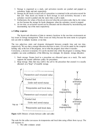
27.  As a program is compiled, each of these high level data structure accesses expands into a
number of low-level pointer arithmetic operations, such as the computation of the
location of the (i, j)th element of a matrix A.
 Accesses to the same data structure often share many common low-level operations.
Programmers are not aware of these low-level operations and cannot eliminate the
redundancies themselves.

2 A Running Example: Quicksort
Consider a fragment of a sorting program called quicksort to illustrate several important
code improving transformations. The C program for quicksort is given below
void quicksort(int m, int n)
/* recursively sorts a[m] through a[n] */
{
int i, j;
int v, x;
if (n <= m) return;
/* fragment begins here */
i=m-1; j=n; v=a[n];
while(1) {
do i=i+1; while (a[i] < v);
do j = j-1; while (a[j] > v);
i f (i >= j) break;
x=a[i]; a[i]=a[j]; a[j]=x; /* swap a[i], a[j] */
}
x=a[i]; a[i]=a[n]; a[n]=x; /* swap a[i], a[n] */
/* fragment ends here */
quicksort (m, j); quicksort (i+1, n) ;
}
Figure 5.1: C code for quicksort
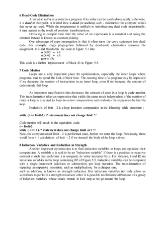
Intermediate code for the marked fragment of the program in Figure 5.1 is shown in
Figure 5.2. In this example we assume that integers occupy four bytes. The assignment x = a[i]
is translated into the two three address statements t6=4*i and x=a[t6] as shown in steps (14) and
(15) of Figure. 5.2. Similarly, a[j] = x becomes t10=4*j and a[t10]=x in steps (20) and (21).
Figure 5.2: Three-address code for fragment in Figure.5.1

28. Figure 5.3: Flow graph for the quicksort fragment of Figure 5.1
Figure 5.3 is the flow graph for the program in Figure 5.2. Block B1 is the entry node. All
conditional and unconditional jumps to statements in Figure 5.2 have been replaced in Figure 5.3
by jumps to the block of which the statements are leaders. In Figure 5.3, there are three loops.
Blocks B2 and B3 are loops by themselves. Blocks B2, B3, B4, and B5 together form a loop, with
B2 the only entry point.
3 Semantics-Preserving Transformations
There are a number of ways in which a compiler can improve a program without
changing the function it computes. Common subexpression elimination, copy propagation, dead-
code elimination, and constant folding are common examples of such function-preserving (or
semantics preserving) transformations.
(a) Before (b)After
Figure 5.4: Local common-subexpression elimination
Some of these duplicate calculations cannot be avoided by the programmer because they
lie below the level of detail accessible within the source language. For example, block B5 shown

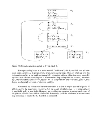
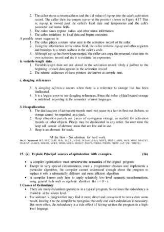
29. in Figure 5.4(a) recalculates 4 * i and 4 *j, although none of these calculations were requested
explicitly by the programmer.
4 Global Common Subexpressions
An occurrence of an expression E is called a common subexpression if E was previously
computed and the values of the variables in E have not changed since the previous computation.
We avoid re-computing E if we can use its previously computed value; that is, the variable x to
which the previous computation of E was assigned has not changed in the interim.
The assignments to t7 and t10 in Figure 5.4(a) compute the common subexpressions 4 *
i and 4 * j, respectively. These steps have been eliminated in Figure 5.4(b), which uses t6
instead of t7 and t8 instead of t10.
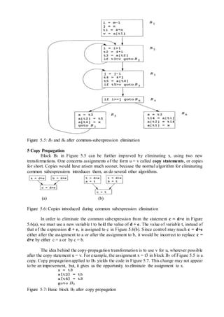
Figure 9.5 shows the result of eliminating both global and local common subexpressions
from blocks B5 and B6 in the flow graph of Figure 5.3. We first discuss the transformation of B5
and then mention some subtleties involving arrays.
After local common subexpressions are eliminated, B5 still evaluates 4*i and 4 * j, as
shown in Figure 5.4(b). Both are common subexpressions; in particular, the three statements
t8=4*j
t9=a[t8]
a[t8]=x
in B5 can be replaced by
t9=a[t4]
a[t4]=x
using t4 computed in block B3. In Figure 5.5, observe that as control passes from the evaluation
of 4 * j in B3 to B3, there is no change to j and no change to t4, so t4 can be used if 4 * j is
needed.
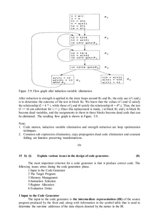
Another common subexpression comes to light in B5 after t4 replaces t8. The new
expression a[t4] corresponds to the value of a[j] at the source level. Not only does j retain its
value as control leaves B3 and then enters B5, but a[j], a value computed into a temporary t5,
does too, because there are no assignments to elements of the array a in the interim. The
statements
t9=a[t4]
a[t6]=t9
in B5 therefore can be replaced by
a[t6]=t5
Analogously, the value assigned to x in block B5 of Figure 5.4(b) is seen to be the same
as the value assigned to t3 in block B2. Block B5 in Figure 5.5 is the result of eliminating
common subexpressions corresponding to the values of the source level expressions a[i] and a[j]
from B5 in Figure 5.4(b). A similar series of transformations has been done to B6 in Figure 5.5.
The expression a[tl] in blocks B1 and B6 of Figure 5.5 is not considered a common
subexpression, although tl can be used in both places. After control leaves B1 and before it
reaches B6, it can go through B5, where there are assignments to a. Hence, a[tl] may not have the
same value on reaching B6 as it did on leaving B1, and it is not safe to treat a[tl] as a common
subexpression.

30. Figure 5.5: B5 and B6 after common-subexpression elimination
5 Copy Propagation
Block B5 in Figure 5.5 can be further improved by eliminating x, using two new
transformations. One concerns assignments of the form u = v called copy statements, or copies
for short. Copies would have arisen much sooner, because the normal algorithm for eliminating
common subexpressions introduces them, as do several other algorithms.
(a) (b)
Figure 5.6: Copies introduced during common subexpression elimination
In order to eliminate the common subexpression from the statement c = d+e in Figure
5.6(a), we must use a new variable t to hold the value of d + e. The value of variable t, instead of
that of the expression d + e, is assigned to c in Figure 5.6(b). Since control may reach c = d+e
either after the assignment to a or after the assignment to b, it would be incorrect to replace c =
d+e by either c = a or by c = b.
The idea behind the copy-propagation transformation is to use v for u, wherever possible
after the copy statement u = v. For example, the assignment x = t3 in block B5 of Figure 5.5 is a
copy. Copy propagation applied to B5 yields the code in Figure 5.7. This change may not appear
to be an improvement, but, it gives us the opportunity to eliminate the assignment to x.
Figure 5.7: Basic block B5 after copy propagation

31. 6 Dead-Code Elimination
A variable is live at a point in a program if its value can be used subsequently; otherwise,
it is dead at that point. A related idea is dead (or useless) code - statements that compute values
that never get used. While the programmer is unlikely to introduce any dead code intentionally,
it may appear as the result of previous transformations.
Deducing at compile time that the value of an expression is a constant and using the
constant instead is known as constant folding.
One advantage of copy propagation is that it often turns the copy statement into dead
code. For example, copy propagation followed by dead-code elimination removes the
assignment to x and transforms the code in Figure 5.7 into
This code is a further improvement of block B5 in Figure 5.5.
7 Code Motion
Loops are a very important place for optimizations, especially the inner loops where
programs tend to spend the bulk of their time. The running time of a program may be improved
if we decrease the number of instructions in an inner loop, even if we increase the amount of
code outside that loop.
An important modification that decreases the amount of code in a loop is code motion.
This transformation takes an expression that yields the same result independent of the number of
times a loop is executed (a loop-invariant computation) and evaluates the expression before the
loop.
Evaluation of limit - 2 is a loop-invariant computation in the following while statement :
while (i <= limit-2) /* statement does not change limit */
Code motion will result in the equivalent code
t = limit-2
while ( i <= t ) /* statement does not change limit or t */
Now, the computation of limit - 2 is performed once, before we enter the loop. Previously, there
would be n + 1 calculations of limit - 2 if we iterated the body of the loop n times.
8 Induction Variables and Reduction in Strength
Another important optimization is to find induction variables in loops and optimize their
computation. A variable x is said to be an "induction variable" if there is a positive or negative
constant c such that each time x is assigned, its value increases by c. For instance, i and t2 are
induction variables in the loop containing B2 of Figure 5.5. Induction variables can be computed
with a single increment (addition or subtraction) per loop iteration. The transformation of
replacing an expensive operation, such as multiplication, by a cheaper one,
such as addition, is known as strength reduction. But induction variables not only allow us
sometimes to perform a strength reduction; often it is possible to eliminate all but one of a group
of induction variables whose values remain in lock step as we go around the loop.

32. Figure 5.8: Strength reduction applied to 4 * j in block B3
When processing loops, it is useful to work "inside-out" ; that is, we shall start with the
inner loops and proceed to progressively larger, surrounding loops. Thus, we shall see how this
optimization applies to our quicksort example by beginning with one of the innermost loops: B3
by itself. Note that the values of j and t4 remain in lock step; every time the value of j decreases
by 1, the value of t4 decreases by 4, because 4 * j is assigned to t4. These variables, j and t4, thus
form a good example of a pair of induction variables.
When there are two or more induction variables in a loop, it may be possible to get rid of
all but one. For the inner loop of B3 in Fig. 9.5, we cannot get rid of either j or t4 completely; t4
is used in B3 and j is used in B4. However, we can illustrate reduction in strength and a part of
the process of induction-variable elimination. Eventually, j will be eliminated when the outer
loop consisting of blocks B2, B3, B4 and Bs is considered.

33. Figure 5.9: Flow graph after induction-variable elimination
After reduction in strength is applied to the inner loops around B2 and B3, the only use of i and j
is to determine the outcome of the test in block B4. We know that the values of i and t2 satisfy
the relationship t2 = 4 * i, while those of j and t4 satisfy the relationship t4 = 4* j. Thus, the test
t2 >= t4 can substitute for i >= j. Once this replacement is made, i in block B2 and j in block B3
become dead variables, and the assignments to them in these blocks become dead code that can
be eliminated. The resulting flow graph is shown in Figure. 5.9.
Note:
1. Code motion, induction variable elimination and strength reduction are loop optimization
techniques.
2. Common sub expression elimination, copy propogation dead code elimination and constant
folding are function preserving transformations.
Or
15 b) (i) Explain various issues in the design of code generator. (8)
The most important criterion for a code generator is that it produce correct code. The
following issues arises during the code generation phase.
1 Input to the Code Generator
2 The Target Program
3 Memory Management
4 Instruction Selection
5 Register Allocation
6 Evaluation Order
1 Input to the Code Generator
The input to the code generator is the intermediate representation (IR) of the source
program produced by the front end, along with information in the symbol table that is used to
determine the run-time addresses of the data objects denoted by the names in the IR.

34. The choice for the intermediate representation includes the following:
 Three-address representations such as quadruples, triples, indirect triples;
 Virtual machine representations such as bytecodes and stack-machine
code;
 Linear representations such as postfix notation.
 Graphical representations such as syntax trees and DAG's.
The front end has scanned, parsed, and translated the source program into a relatively
low-level IR, so that the values of the names appearing in the IR can be represented by quantities
that the target machine can directly manipulate, such as integers and floating-point numbers.
All syntactic and static semantic errors have been detected, that the necessary type
checking has taken place, and that type-conversion operators have been inserted wherever
necessary. The code generator can proceed on the assumption that its input is error free.
2 The Target Program
The output of the code generator is the target program which is going to run in the
following computers.
 The instruction-set architecture of the target machine has a significant impact on the
difficulty of constructing a good code generator that produces high-quality machine code.
The most common target-machine architectures are RISC (reduced instruction set
computer), CISC (complex instruction set computer), and stack based.
 A RISC machine typically has many registers, three-address instructions, simple
addressing modes, and a relatively simple instruction-set architecture. In contrast, a
CISC machine typically has few registers, two-address instructions, a variety of
addressing modes, several register classes, variable-length instructions, and instructions
with side effects.
 In a stack-based machine, operations are done by pushing operands onto a stack and
then performing the operations on the operands at the top of the stack. To achieve high
performance the top of the stack is kept in registers.
 The JVM is a software interpreter for Java bytecodes, an intermediate language
produced by Java compilers. The interpreter provides software compatibility across
multiple platforms, a major factor in the success of Java. To improve the high
performance interpretation just-in-time (JIT) Java compilers have been created.
The output of the code generator may be:
 Absolute machine language program: It can be placed in a fixed memory location and
immediately executed.
 Reloadable machine-language program: It allows subprograms (object modules) to be
compiled separately. A set of relocatable object modules can be linked together and
loaded for execution by a linking loader. the compiler must provide explicit relocation
information to the loader if automatic relocation is not possible.
 Assembly language program: The process of code generation is somewhat easier, but
assembly must be converted into machine executable code with help of assembler.
3 Memory Management
 Names in the source program are mapped to addresses of data objects in run-time
memory by both the front end and code generator.
 Memory Management uses symbol table to get names information.
 The amount of memory required by declared identifies are calculated and storage space
is reserved in memory at run time.
 Labels in three address code are converted into equivalent memory address.

35.  For instance if a reference to “goto j” is encountered in three address code then
appropriate jump instruction can be generated by computing memory address for label j.
 Some instruction address can be calculated in run time only that is also after loading the
program.
4 Instruction Selection
The code generator must map the IR program into a code sequence that can be executed by
the target machine. The complexity of performing this mapping is determined by a factors such
as
 The level of the intermediate representation (IR).
 The nature of the instruction-set architecture.
 The desired quality of the generated code.
If the IR is high level, the code generator may translate each IR statement into a sequence of
machine instructions using code templates. Such statement-by-statement code generation,
however, often produces poor code that needs further optimization. If the IR reflects some of the
low-level details of the underlying machine, then the code generator can use this information to
generate more efficient code sequences.
The uniformity and completeness of the instruction set are important factors. The
selection of instruction depends on the instruction set of the target machine. Instruction speeds
and machine idioms are other important factors in selection of instruction.
If we do not care about the efficiency of the target program, instruction selection is
straightforward. For each type of three-address statement, we can design a code skeleton that
defines the target code to be generated for that construct.
For example, every three-address statement of the form x = y + z, where x, y, and z are
statically allocated, can be translated into the code sequence
LD R0, y // R0 = y (load y into register RO)
ADD R0, R0, z // R0 = R 0 + z (add z to R0)
ST x, R0 // x = R0 (store RO into x)
This strategy often produces redundant loads and stores. For example, the sequence of three-
address statements
a = b + c
d = a + e
would be translated into the following code
LD R0, b // R0 = b
ADD R0, R0, c // R0 = R0 + c
ST a, R0 // a = R0
LD R0, a // R0 = a
ADD R0, R0, e // R0 = R0 + e
ST d, R0 // d = R0
Here, the fourth statement is redundant since it loads a value that has just been stored, and so is
the third if a is not subsequently used.
The quality of the generated code is usually determined by its speed and size. On most
machines, a given IR program can be implemented by many different code sequences, with
significant cost differences between the different implementations. A naive translation of the
intermediate code may therefore lead to correct but unacceptably inefficient target code.
5 RegisterAllocation
A key problem in code generation is deciding what values to hold in what registers.
Registers are the fastest computational unit on the target machine, but we usually do not have
enough of them to hold all values. Values not held in registers need to reside in memory.

36. Instructions involving register operands are invariably shorter and faster than those involving
operands in memory, so efficient utilization of registers is particularly important.
The use of registers is often subdivided into two subproblems:
1. Register allocation: During register allocation, select the appropriate set of variables
that will reside in registers at each point in the program.
2. Register assignment: During register assignment, pick the specific register in which
corresponding variable will reside in.
Finding an optimal assignment of registers to variables is difficult, even with single-
register machines. Mathematically, the problem is NP-complete. The problem is further
complicated because the hardware and/or the operating system of the target machine may require
that certain register-usage conventions be observed. Certain machines require register-pairs for
some operands and results.
Consider the two three-address code sequences, the only difference is the operator in the second
statement.
t = a + b
t = t * c
t = t / d
The efficient Optimal machine-code sequences with only one register R0
LD R0, a
ADD R0, b
MUL R0, c
DIV R0, d
ST R0, t
6 Evaluation Order
The evaluation order is an important factor in generating an efficient target code. Some
computation orders require fewer registers to hold intermediate results than others. However,
picking a best order in the general case is a difficult NP-complete problem. We can avoid the
problem by generating code for the three-address statements in the order in which they have
been produced by the intermediate code generator.
(ii) Write note on Simple code generator. (8)
A code generator generates target code for a sequence of three-address instructions. One
of the primary issues during code generation is deciding how to use registers to best advantage.
Best target code will use minimum registers in execution.
There are four principal uses of registers:
 The operands of an operation must be in registers in order to perform the operation.
 Registers make good temporaries - used only within a single basic block.
 Registers are used to hold (global) values that are computed in one basic block and
used in other blocks
 Registers are often used to help with run-time storage management
The machine instructions are of the form
 LD reg, mem
 ST mem, reg
 OP reg, reg, reg
Registerand Address Descriptors
 For each available register, a register descriptor keeps track of the variable names
whose current value is in that register. Initially all register descriptors are empty. As
the code generation progresses, each register will hold the value.

37.  For each program variable, an address descriptor keeps track of the location or
locations where the current value of that variable can be found. The location might be
a register, a memory address, a stack location, or some set of more than one of these.
The information can be stored in the symbol-table entry for that variable name.
Function GetReg
 An essential part of the algorithm is a function getReg(I), which selects registers for
each memory location associated with the three-address instruction I.
 Function getReg has access to the register and address descriptors for all the variables
of the basic block, and may also have access to certain useful data-flow information
such as the variables that are live on exit from the block.
 In a three-address instruction such as x = y + z, A possible improvement to the
algorithm is to generate code for both x = y + z and x = z + y whenever + is a
commutative operator, and pick the better code sequence.
Machine Instructions for Operations
For a three-address instruction with Operations (+, - , * , / , …) such as x = y + z, do the
following:
1. Use getReg(x = y + z) to select registers for x, y, and z. Call these Rx, Ry, and Rz.
2. If y is not in Ry (according to the register descriptor for Ry), then issue an instruction
LD Ry, y', where y' is one of the memory locations for y (by the address descriptor for
y).
3. Similarly, if z is not in Rz, issue and instruction LD Rz, z', where z' is a location for z .
4. Issue the instruction ADD Rx, Ry, Rz.
Machine Instructions for Copy Statements
 Consider an important special case: a three-address copy statement of the form x = y.
 We assume that getReg will always choose the same register for both x and y. If y is
not already in that register Ry, then generate the machine instruction LD Ry, y.
 If y was already in Ry, we do nothing.
Managing Registerand Address Descriptors
As the code-generation algorithm issues load, store, and other machine instructions, it
needs to update the register and address descriptors. The rules are as follows:
1. For the instruction LD R, x
a. Change the register descriptor for register R so it holds only x.
b. Change the address descriptor for x by adding register R as an additional location.
2. For the instruction ST x, R, change the address descriptor for x to include its own
memory location.
3. For an operation OP R, R, R such as ADD Rx, Ry, and Rz implementing a three-
address instruction x = y + x
a. Change the register descriptor for Rx so that it holds only x.
b. Change the address descriptor for x so that its only location is Rx. Note that the
memory location for x is not now in the address descriptor for x.
c. Remove Rx from the address descriptor of any variable other than x.
4. When we process a copy statement x = y, after generating the load for y into register
Ry, if needed, and after managing descriptors as for all load statements (per rule I):
a. Add x to the register descriptor for Ry.
b. Change the address descriptor for x so that its only location is Ry.

38. Example 5.16 : Let us translate the basic block consisting of the three-address statements
t = a – b
u = a – c
v = t + u
a = d
d = v + u where t, u, and v are temporaries, local to the block, while a, b, c, and d
are variables that are live on exit from the block. When a register's value is no longer needed,
then we reuse its register. A summary of all the machine-code instructions generated is in
Figure.
All the Best – No substitute for hard work.
Mr. G. Appasami SET, NET, GATE, M.Sc., M.C.A., M.Phil., M.Tech., (P.hd.), MISTE, MIETE, AMIE, MCSI, MIAE, MIACSIT,
MASCAP, MIARCS, MISIAM, MISCE, MIMS, MISCA, MISAET, PGDTS, PGDBA, PGDHN, PGDST, (AP / CSE / DRPEC).