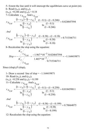
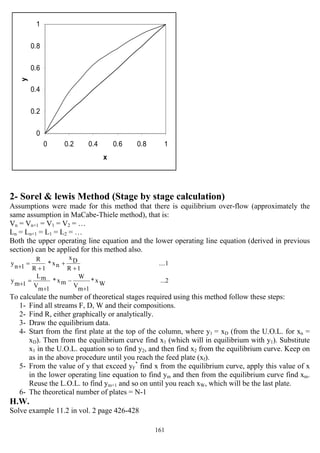
1. Mass transfer is the movement of a component from one location to another where the concentration is different. It occurs through molecular diffusion and eddy diffusion.
2. Molecular diffusion is the random movement of molecules due to thermal motion. Eddy diffusion is the random macroscopic fluid motion in turbulent flows.
3. Fick's first law states that the rate of molecular diffusion is proportional to the concentration gradient. The rate of mass transfer stops when concentrations are uniform.

(X[
Z-Z
D.C
n 212
22
2 NN
12
HN
N =
)10*(7.85
15
)25.08.0)(784.0)(10*(4.09
n 3-
-5
N2
−
=
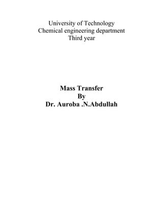
2Nn = 9.23 X 10⁻⁹
mol/s in the positive Z direction
2Hn = 9.23 X 10⁻⁹
mol/s in the negative Z direction
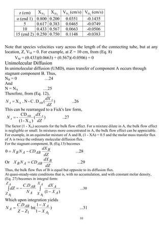
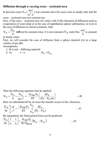
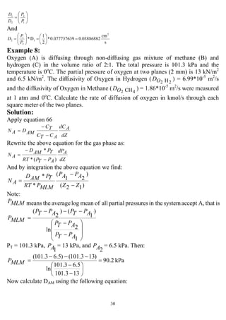
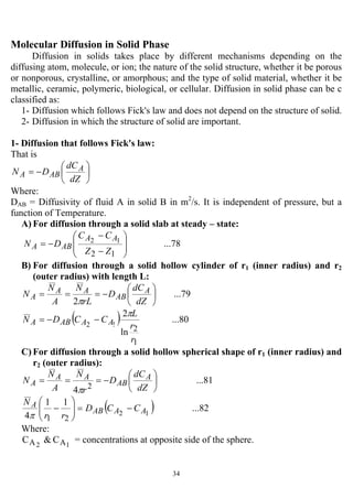
(b)For equimolar counter diffusion, the molar average velocity of the mixture, VM, is
Zero
Therefore, from (Eq. 9), species velocities are equal to species diffusion velocities.
Thus,
)])(10*09.4)(10*[(7.85
10*9.23
XCA
n
C
J
)(VV
22
2
2
2
22 55-
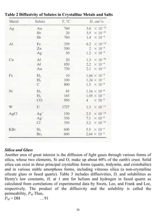
-9
N
N
N
N
NN
N
D
X−
====
)(
0.0287
V
2
2N
NX
= in the positive Z direction
Similarly
)(
0.0287
V
2
2H
HX
= in the negative Z direction
Thus, species velocities depend on species mole fractions, as follows:](https://image.slidesharecdn.com/masstransferdrauroba-150501120755-conversion-gate01/85/Mass-transfer-dr-auroba-11-320.jpg)
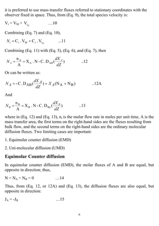
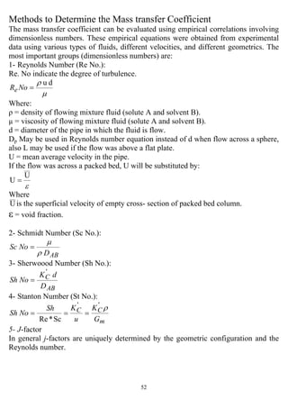
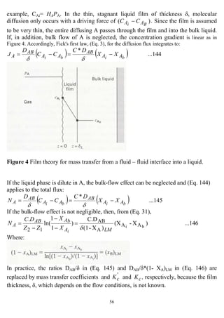
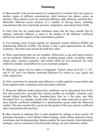
![13
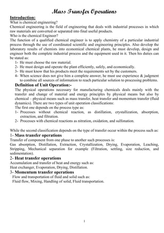
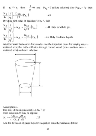
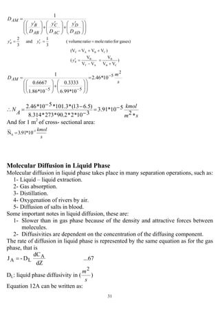
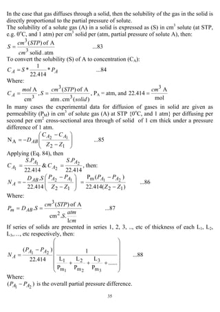
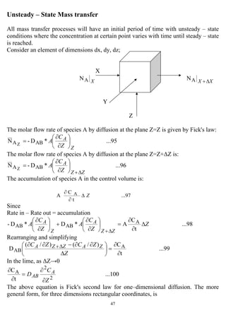
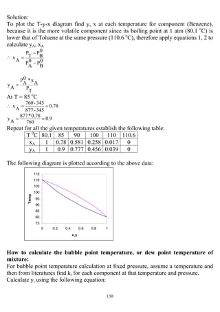
(c) The initial fractions of the mass transfer fluxes due to molecular diffusion.
(d) The initial diffusion velocities, and the species velocities (relative to stationary coordinates) in
the stagnant layer.
(e) The time in hours for the benzene level in the beaker to drop 2 cm from the initial level, if the
specific gravity of liquid benzene is 0.874. Neglect the accumulation of benzene and air in the
stagnant layer as it increases in height.
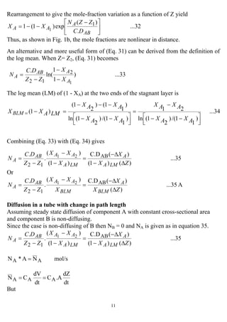
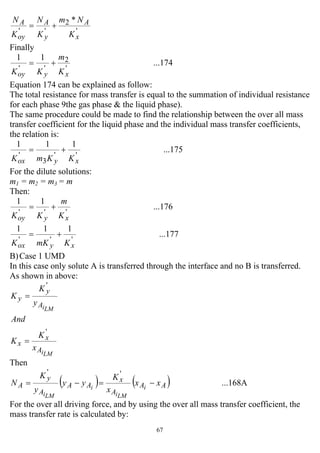
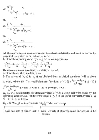
Figure 2 Evaporation of Benzene from a beaker
SOLUTION:
Let A = benzene, B = air.
3
5-
cm
mol
10*4.09
8)(82.06)(29
1
T.R
P
C ===
(a) Take Zl = 0.
Then Z2 - Zl = ∆Z = 0.5 cm.
From Dalton's law, assuming equilibrium at the liquid benzene-air interface,
0.131
1
0.131
P
P 1
1
A
===AX
02
=AX
Then
[ ]
0.933
0.131)-(1/0)-(1ln
0.131
)X-(1 A ===BLMX
From equation 35, or Equation 35A](https://image.slidesharecdn.com/masstransferdrauroba-150501120755-conversion-gate01/85/Mass-transfer-dr-auroba-15-320.jpg)
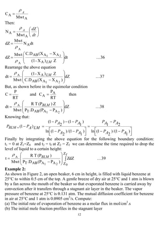
![14
s.mol/cm10*1.04
933.0
131.0
5.0
)0905.0)(10*(4.09
N 26-
5-
A =⎟
⎠
⎞
⎜
⎝
⎛
=
(b)
Z0.281
)0905.0)(10*09.4(
)0)(10*(1.04
C.D
(N
5
6-
AB
)1A
=
−
=
−
−
ZZZ
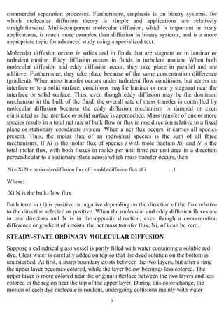
From equation 32,
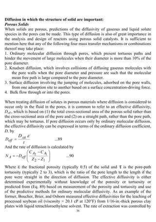
XA = 1 – 0.869[exp (0.281Z)] (1)
Using the above equation (1), the following results are obtained:
These profiles are only slightly curved.
(c) From (Eq. 27) and (Eq. 29), we can compute the bulk flow terms, XANA and
XBNA, from which the molecular diffusion (Ji) terms are obtained.
Note that the molecular diffusion fluxes are equal but opposite, and the bulk flow flux
of B is equal but opposite to its molecular diffusion flux, so that its molar flux, NB, is
zero.
(d) From (Eq. 6)
(2)cm/s0254.0
10*4.09
10*1.04
C
N
C
N
V
5-
6-
A
M ====](https://image.slidesharecdn.com/masstransferdrauroba-150501120755-conversion-gate01/85/Mass-transfer-dr-auroba-16-320.jpg)
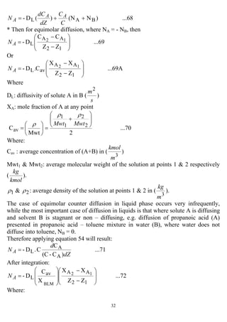
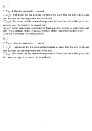
![20
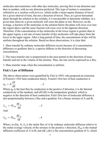
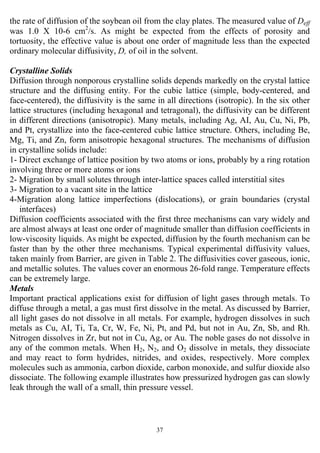
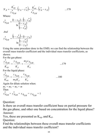
Table (1) Diffusion Volumes from Fuller, Ensley, and Giddings [J. Phys. Chem.,
73, 3679-3685 (1969)] for Estimating Binary Gas Diffusivity by the Method of
Fuller et al.
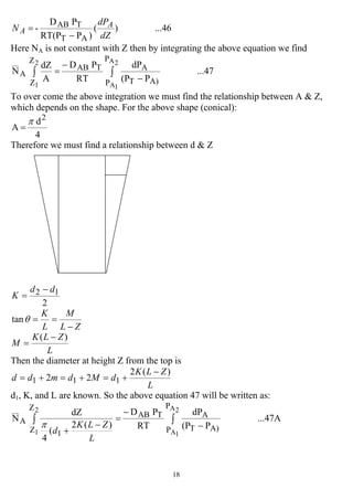
From equation (50) we can notice that:
P
1.75
T
Dα
And:
...52
1
2
75.1
2
1
2
1
⎟⎟
⎠
⎞
⎜⎜
⎝
⎛
⎟⎟
⎠
⎞
⎜⎜
⎝
⎛
=
P
P
T
T
D
D](https://image.slidesharecdn.com/masstransferdrauroba-150501120755-conversion-gate01/85/Mass-transfer-dr-auroba-22-320.jpg)
![26
sec
10*722.162.0
R*lbmol
ftatm
0.7302RUse
atm908.0
822.0
1
ln
822.01
ln
P
atm1Hgmm7600-760P
atm0.822mmHg625135760P
2
4
2
3
BLM
B
B
1
2
22
2
1
ft
hr
ft
D
P
P
PP
AB
B
B
BB
−
==
=
=
−
=
−
=
===
==−=
Now by integrating the above equation, we find:
[ ]
sec
lbmol
10*111.8
)
6
1
4
1
(
0178.0
*
908.0*537*7302.0
1*10*722.1
4
N
*
*
6
1
6
1N*4
7
4
A
1
12
A
2
−
−
=
⎟
⎟
⎟
⎟
⎠
⎞
⎜
⎜
⎜
⎜
⎝
⎛
−
−
⎥
⎥
⎦
⎤
⎢
⎢
⎣
⎡
=
−=⎥
⎦
⎤
⎢
⎣
⎡
−
−
−
π
π
AA
BLM
TAB PP
PRT
PD
ZZ
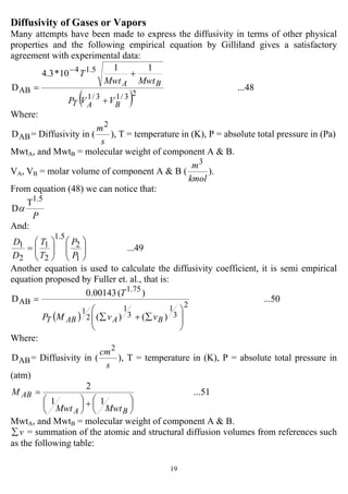
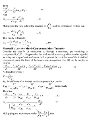
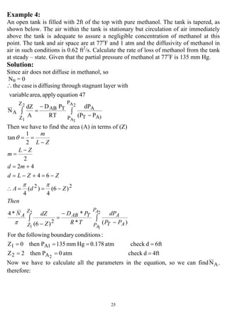
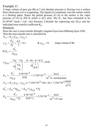
Example 5:
A small diameter tube closed at one end was filled with acetone to within 18 mm of
the top and maintained at 290 K and 99.75 kPa with a gentle stream of air blowing
across the top. After 15 ksec, the liquid level had fallen to 27.5 mm. The vapor
pressure of acetone at that temperature is 21.95 kN/m2
. Calculate the diffusivity of
acetone in air, given the following data:
Mwt of acetone = 58
The density of acetone (ρ) = 790 kg/m3
Solution:
Since evaporation is occurred through constant area, then apply equation 39 and by
integrating this equation we find:
⎟
⎟
⎠
⎞
⎜
⎜
⎝
⎛
−
⎟
⎟
⎠
⎞
⎜
⎜
⎝
⎛
−
=
22
Z
)PP(.DP
)(PTR
Mwt
t
2
0
2
f
AAABT 21
A
ZBLM
ρ
To apply this equation we must first calculate each parameter in the equation as:
PT = 99.75 kPa
T = 290 K
K*kmol
m*kPa
314.8
3
=R](https://image.slidesharecdn.com/masstransferdrauroba-150501120755-conversion-gate01/85/Mass-transfer-dr-auroba-28-320.jpg)
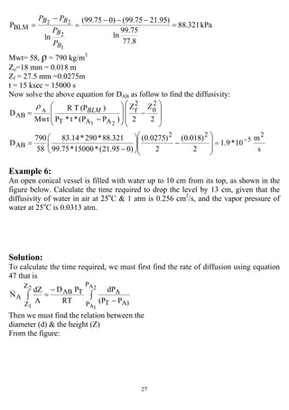
![49
( ) ...106n 00ZA AA
AB CCA
t
D
s
−==
π
We can determine the total number of moles of solute, NA, transferred into the semi-
infinite medium by integrating equation 106 with respect to time:
( ) ...107)(2 00
00
0
ππ
tD
CCA
t
dt
CCA
D
dtn AB
AA
t
AA
AB
t
zA ss
−=−== ∫∫ =AN
Medium of finite Thickness with Sealed Edges
Consider a rectangular parallelepiped medium of finite thickness 2a in the Z direction,
and either infinitely long dimensions in the y and x directions or finite lengths of 2b
and 2c respectively, in those directions. The boundary conditions for this case to solve
(Equ.100)
2
2
A
t
C
Z
C
D A
AB
∂
∂
=
∂
∂
are:
At t = 0 -a < Z < a CA = CA0
t = 0 Z = ± a CA = CAs (CAs > CA0)
t > 0 Z = 0
t
CA
∂
∂
= 0
again by the method of separation of variables or the Laplace transform method the
result in terms of the fractional unaccomplished concentration change, E, is
[ ] ...108
2
)12(
cos
0
2
4/
22
)12(exp
)12(
)1(4
1
a
Zn
n
atnABD
n
n
oAC
sAC
AC
sAC
E
π
π
π
θ
+
∑
∞
=
+−
+
−
=
−
−
=−=
or, in terms of complementary error function,
...109
0n 2
)12(
2
)12(
)1(1 ∑
∞
=
++
+
−+
−=
−
−
=−=
⎥
⎥
⎦
⎤
⎢
⎢
⎣
⎡
tABD
Zan
erfc
tABD
Zan
erfcn
oAC
sAC
AC
sAC
E θ
The instantaneous rate of mass transfer across the surface of either unsealed face of the
medium (i.e. at Z = ± a), is obtained by differentiating (Eq. 108, or 109) with respect
to Z, evaluating the result at Z = a, followed by substitution into Fick's first law to give
( )
...110
4
)12(
exp
2
0
2
22
∑
∞
=
=
⎥
⎥
⎦
⎤
⎢
⎢
⎣
⎡ +
−
−
=
n
ABAAAB
aZA
a
tnD
a
ACCD
n os π
We can also determine the total number of moles transferred across either unsealed
face by integrating (Eq. 110) with respect to time. Thus
...111
2
4
22
)12(
exp1
0 2
)12(
1
2
)(8
0 ⎪⎭
⎪
⎬
⎫
⎪⎩
⎪
⎨
⎧
⎥
⎥
⎦
⎤
⎢
⎢
⎣
⎡ +
−−∑
∞
= +
−
=∫ ==
a
tnABD
n n
Aa
oAC
sACt
dtaZAnAN
π
π](https://image.slidesharecdn.com/masstransferdrauroba-150501120755-conversion-gate01/85/Mass-transfer-dr-auroba-51-320.jpg)
![82
Chapter Three
Absorption and Stripping
Introduction:
In absorption (also called gas absorption, gas scrubbing, and gas washing), a gas
mixture is contacted with a liquid (the absorbent or solvent) to selectively dissolve one
or more components by mass transfer from the gas to the liquid. The components
transferred to the liquid are referred to as solute or absorbate.
Absorption is used to separate gas mixture; remove impurities, contaminants,
pollutants, or catalyst poisons from gas; or recovery valuable chemicals. Thus, the
species of interest in the gas mixture may be all components, only the component(s)
not transferred, or only the component(s) transferred.
The opposite of absorption is stripping (also called de-sorption), wherein a liquid
mixture is contacted with gas to selectively remove components by mass transfer from
the liquid to the gas phase.
The absorption process involves molecular and turbulent diffusion or mass transfer of
solute [A] through a stagnant layer gas [B] then through non – diffusing liquid [C].
There are two types of absorption processes:
1- Physical process (e.g. absorption of acetone from acetone – air mixture by water.
2- Chemical process, sometimes called chemi-sorption (e.g. absorption of nitrogen
oxides by water to produce nitric acid.
Equipment:
Absorption and stripping are conducted in tray towers (plate column), packed column,
spray tower, bubble column, and centrifugal contactors. The first two types of these
equipment will be considered in our course for this year.
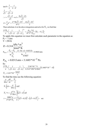
1- Tray tower:
A tray tower is a vertical, cylindrical pressure vessel in which vapor and liquid, which
flow counter currently, are contacted on a series of metal trays or plates. Liquid flows
across any tray over an outlet weir, and into a down comer, which takes the liquid by
gravity to the tray below. The gas flows upward through opening in each tray,
bubbling through the liquid on the other tray. A schematic diagram for the flow
patterns inside the tray column is shown below.
In Chemical Engineering vol. 2 by J. M. Coulson & J. F. Richardson a review for the
types of trays used in plate towers are given in page 573.](https://image.slidesharecdn.com/masstransferdrauroba-150501120755-conversion-gate01/85/Mass-transfer-dr-auroba-84-320.jpg)
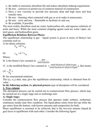
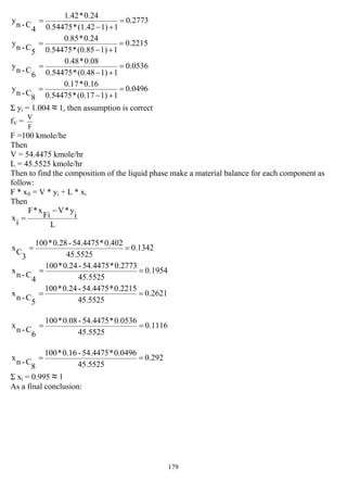
![85
LT GT
xT yT
LB GB
xB yB
Where:
L: moles of liquid phase/ unit time
G: moles of gas phase/ unit time
We will denote the streams in the top of the equipment by (T), and those in the bottom
of the equipment by (B).
Then, the overall material balance equation for the above consideration can be written
as:
T
G
B
L
B
G
T
L +=+
(Mole balance can be used because there is no chemical reaction)
[A] M.B.
T
y*
T
G
B
x*
B
L
B
y*
B
G
T
x*
T
L +=+
Where:
x: is the mole fraction of solute A in the liquid phase.
y: is the mole fraction of solute A in the gas phase.
Since only component A is redistributed between the two phases then, a balance
component for A can be written as follow:
)
T
y-1
T
y
(`G)
B
x-1
B
x
(`L)
B
y-1
B
y
(`G)
T
x-1
T
x
(`L +=+
The above equation is called the operating equation where:
`L : Moles of inert liquid (solute–free absorbent) / unit time
`G : Mole of inert gas {solute–free gas (or career gas)} / unit time
The operating equation can also be written as:
T
Y*`G
B
X*`L
B
Y*`G
T
X*`L +=+
Where:
phaseliquidin the(inerts)componentsA-nonmoles
phaseliquidin theAsoluteofmoles
x-1
x
X ==
Single stage](https://image.slidesharecdn.com/masstransferdrauroba-150501120755-conversion-gate01/85/Mass-transfer-dr-auroba-87-320.jpg)

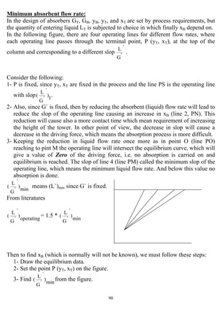
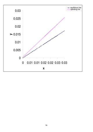
![93
Algebraic method for determining the number of equilibrium stages:
Graphical methods for determining equilibrium stages have great educational value
because of fairly complex multistage problem can be readily followed and understood.
Furthermore, one can quickly gain visual insight into the phenomena involved.
However, the application of graphical method can become very tedious when (1) the
problem speciation fixes the number of stages rather than the percent recovery of
solute, (2) when more than one solute is being absorbed or stripped, (3) when the best
operating conditions of temperature and pressure are to be determined so that the
location of the equilibrium curve is unknown, and/or (4) if very low or very high
concentrations force the graphical construction to the corners of the diagram so that
multiple y – x diagrams of varying sizes and dimensions are needed. Then the
application of an algebraic method may be preferred.
When the flow rate of L and G are constant and the process is countercurrent and the
equilibrium line is a straight line and can be presented by the relation y = m* x, also if
the operating line is a straight line (i.e. dilute solution), a simplified analytical equation
found by Kremser et al. can be used to find the number of theoretical plates as follow:
1- For absorption:
1-1NA
A-1NA
*
T
y-
B
y
T
y
B
y
+
+
=
−
Then
Alog
]
A
1
)
A
1
-1(
T
x*m-
T
y
T
x*m-
B
y
log[
N
+
=
Where
N: Theoretical number of plates.
T
x*m*
T
y = (Equilibrium relation for dilute solution)
A: absorption factor which is the ratio of slop of operating line ( G
L ) to the slop of
equilibrium line (m), then:
G*m
L
A =
For high degree of absorption (high % recovery):
1- Use large number of plates.
2- Use high absorption factor (A), since m is constant by the system, then to get
high value of A means ( G
L ) must be larger than m.
The most economic value of A is about (1.3) {suggested by Calburn}.](https://image.slidesharecdn.com/masstransferdrauroba-150501120755-conversion-gate01/85/Mass-transfer-dr-auroba-95-320.jpg)
![94
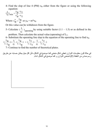
2- For stripping:
1-1N)
A
1
(
)
A
1
(-1N)
A
1
(
)
m
B
y
(-
T
x
B
x
T
x
+
+
=
−
And
)
A
1
(log
A])A-1(
)m
B
y
(-
B
x
)m
B
y
(-
T
x
log[
N
+
=
Where:
*
B
x
m
B
y
=
ﺔاﻟﻬﻨﺪﺳ ﺎبآﺘ ﺑﻤﺮاﺟﻌﺔ ﻋﻠﻴﻪ اﻻﻃﻼع ﻳﻤﻜﻦ و اﻟﺼﻮاﻧﻲ ﻋﺪد ﺣﺴﺎب ﻓﻲ اﻟﻤﺴﺘﺨﺪﻣﺔ ﻟﻠﻤﻌﺎدﻻت ﻣﻄﻠﻮﺑﺔ اﻻﺷﺘﻘﺎﻗﺎت
اﻟﻜﻴﻤﻴﺎوﻳﺔ)اﻟﺜﺎﻧﻲ اﻟﺠﺰء(اﻟﺼﻔﺤﺔ573.Chemical engineering (vol. 2) by J. M.Coulson &J. F.
Richardson
Example 2:
When molasses is fermented to produce a liquor containing ethyl alcohol, a CO2- rich
vapor containing a small amount of ethyl alcohol is evolved. The alcohol can be
recovered by absorption with water in a sieve-tray tower. For the following conditions,
determine the number of equilibrium stages required for countercurrent flow of liquid
and gas, assuming isothermal, isobaric conditions in the tower and neglecting mass
transfer of all components except ethyl alcohol.
Entering gas:
180 kmole/hr; 98 mol% CO2, 2 mol% ethyl alcohol; 30 o
C, 110 kPa
Entering liquid absorbent:
100 % water; 30 o
C, 110 kPa
Required recovery (absorption) of ethyl alcohol (R): 97%
Equilibrium relationship: y = 0.57*x
Solution:
YT = (1- R) * YB
0.02041
0.02-1
0.02
B
y-1
B
y
B
Y ===
yT = 0.03 * 0.02041 = 0.00061 (mole fraction of ethyl alcohol in the top)
*
B
x = yB/m = 0.02/0.57 = 0.03509](https://image.slidesharecdn.com/masstransferdrauroba-150501120755-conversion-gate01/85/Mass-transfer-dr-auroba-96-320.jpg)
![98
Calculations of the height of packing: x T yT
A- for dilute mixtures LT GT
Consider the following figure, then
O. M. B. on the denoted section
G)dLL()dGG(L ++=++
dLdG =∴
[A] M. B.:
A
A
N
A
N =
d (G* y) = d (L*x)
LB GB
xB yB
A
Ny)*(Gd =Θ
And
or
dAyykN iyA )( −=Θ
dAyykN oyA )( *
−=
Then
dAyykGyd
or
dAyykGyd
oy
iy
)()(
)()(
*
−=
−=
Where:
dA: is the interfacial area associated with differential tower length, it is very difficult
to measure in packed towers so, for packed towers
dA = a*s*dZ
Where:
a: Specific interfacial area per unit volume of packing (m2
/m3
)
s: empty tower cross-sectional area (m2
)
dZ: differential height in (m)
Then:
sdzyyaksdzyyakGyd oyiy )()()( *
−=−=
So
∫∫∫ −
=
−
=
B
T
B
T
y
y oy
y
y iy
Z
syyak
Gyd
syyak
Gyd
dZ
)(
)(
)(
)(
*
0
In absorption of dilute solution the flow rate does not effected by the small change in
concentration, so
2
B
G
T
G
mGG
+
== (i.e. constant through out the column)](https://image.slidesharecdn.com/masstransferdrauroba-150501120755-conversion-gate01/85/Mass-transfer-dr-auroba-100-320.jpg)
![107
90.00253145
0*0.57-0.00061
0.0234*0.57-0.02
ln(
0)*0.57-(0.00061-0.0234)*0.57-(0.02
)y(y
)y(y
ln
)y(y)y(y
)y(y
*
TT
*
BB
*
TT
*
BB
m
*
==
−
−
−−−
=−
7.66
90.00253145
0.00061-0.02
oy(NTU) ==∴
Z = (HTU)oy * (NTU)oy = 2 * 7.66 = 15.32 ft
Example 4:
Experimental data have been obtained for air containing 1.6 vol% SO2 being scrubbed
with pure water in a packed column of 1.5 m2
in cross-sectional area and 3.5 m in
packed height. Entering gas and liquid flow rates are 0.062 and 2.2 kmole/sec,
respectively. If the outlet mole fraction of SO2 in the gas is 0.004 and column
temperature is near ambient, calculate from the data:
(a) The (NTU)oy for absorption of SO2
(b) The (HTU)oy in meters
(c) The volumetric overall mass transfer coefficient, koya for SO2 in (kmole/m3
s
mole fraction)
Solution
(a) First we must find xB
[SO2] O.M. B.
T
y*
T
G
B
x*
B
L
B
y*
B
G
T
x*
T
L +=+
And finally
T
Y*`G
B
X*`L
B
Y*`G
T
X*`L +=+
L`= LT (because xT = 0)
L` = 2.2 kmole/s
G` = GB *(1- yB) = 0.062 * (1- 0.016) = 0.061008 kmole/s
Then
2.2
20.00024501-0.0009920
2.2
)]
0.004-1
0.004
(*[0.061008-)]
0.016-1
0.016
(*0.061008[)0*
T
(L
B
X
+
=
+
= XB
= 0.00034
Then
xB = 0.00034 (dilute solution XB = xB)
(NTU)oy=
m
TB
y
y yy
yy
yy
dyB
T
)( **
−
−
=
−∫
40.00313218
)
0*40-0.004
0.00034*40-0.016
ln(
0)*40-(0.004-)0.00034*40-(0.016
)y(y
)y(y
ln
)y(y)y(y
)y(y
*
TT
*
BB
*
TT
*
BB
m
*
==
−
−
−−−
=−
3.8312
40.00313218
0.004-0.016
oy(NTU) ==∴
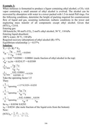
(b) Z = (HTU)oy * (NTU)oy](https://image.slidesharecdn.com/masstransferdrauroba-150501120755-conversion-gate01/85/Mass-transfer-dr-auroba-109-320.jpg)
![108
(HTU)oy = Z / (NTU)oy= 3.5/3.8312 = 0.9136 m
(c)
ask
G
(HTU)
oy
m
oy =
fractionmoleSec3m
kmole
0.045245
1.5*0.9136
0.062
soy(HTU)
mG
aoyk ===∴
Example 5:
Acetone is being absorbed by water in a packed tower having a cross-sectional area of
0.186 m2
at 293 k and 101.3 kPa. The inlet air contains 2.6 mol% acetone and the out
let 0.5 mol%. The gas flow rate is 13.65 kmole air inlet/ hr. The pure water inlet flow
rate is 45.36 kmole/ hr. The film coefficients for the given conditions in the tower are:
fractionmole.packing3m.Sec
komle2-3.78x10a`
yk =
fractionmole.packing3m.Sec
komle2-6.16x10a`
xk =
The equilibrium data is given by the equation: (y = 1.186 x)
Calculate the height of packing using:
(a) a`
yk
(b) a`
xk
Also calculate ( a`
oyk ) and the height of packing based on this coefficient.
Solution:
(a) Z = (HTU)y * (NTU)y
Where:
(NTU)y =
mi
TB
y
y i yy
yy
yy
dyB
T
)( −
−
=
−∫
And
)(
)(
ln
)()(
)(
TiT
BiB
TiTBiB
mi
yy
yy
yyyy
yy
−
−
−−−
=−
Also (HTU)y =
as`
yk
mG
Then we have to find xB so then we can find each of xiB, yiB, xiT, and yiT
[A] M. B.
T
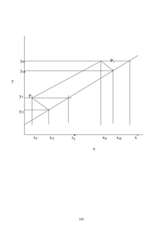
y*`G
B
x*`L
B
y*`G
T
x*`L +=+ (Dilute solution)
L`= LT = 45.31 kmole/hr (xT = 0)
G` = 13.65 kmole/hr (given in data)
Then:
0.00632
45.36
13.65)*(0.00513.65)*(0.02645.36)*(0
B
x =
−+
=](https://image.slidesharecdn.com/masstransferdrauroba-150501120755-conversion-gate01/85/Mass-transfer-dr-auroba-110-320.jpg)
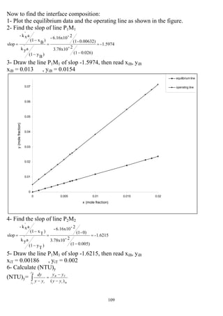
![114
Where:
f(y) =
)
i
y(y2y)(1
im
y
a`
yk
1
−−
7-
8- Plot f(y) vs. (y) and then calculate the area under the curve starting from yB to yT.
To calculate the area under the curve. There are two methods:
(a) By counting the squares formed and multiply the number of squares by the area of
each square as shown below.
(b) Using Simpson's rule:
]))2nf(y..)6f(y)4f(y)22(f(y))12nf(y..)5f(y)3f(y)14(f(y))nf(y)0[(f(y
3
h
Area ++++++++++++=
As shown below.](https://image.slidesharecdn.com/masstransferdrauroba-150501120755-conversion-gate01/85/Mass-transfer-dr-auroba-116-320.jpg)
![116
Θان ﻳﻌﻨﻲ ﻣﻤﺎ ﻣﺒﺎﺷﺮة ﻳﺤﺼﻞ اﻟﺘﻔﺎﻋﻞ)B(اﻟﻐﺎز ﻳﺴﺘﺪﻋﻲ ﻣﻤﺎ اﻟﺴﺎﺋﻞ ﻃﺒﻘﺔ ﻓﻲ ﻳﻨﺘﻬﻲ)A(ﺔﻃﺒﻘ ﻲﻓ ﺸﺎرﻟﻼﻧﺘ
اﺧﺮى ﻃﺒﻘﺔ ﻟﺬﻟﻚ ﺗﺘﻜﻮن و اﻟﺴﺎﺋﻞ)اﻟﺘﻔﺎﻋﻞ ﻣﻨﻄﻘﺔ(ﺰﺗﺮآﻴ ﻮنﻳﻜ ﺎهﻨ و ﻞاﻟﺘﻔﺎﻋ ﺎﻓﻴﻬ ﺪثﻳﺤ اﻟﺘﻲ ة اﻟﺴﺎﺋﻞ ﻃﺒﻘﺔ ﻓﻲ
AوBﺻﻔﺮ.ﻟﻠﻤﺎدة ﺗﺮآﻴﺰ اﻋﻠﻰ ان)AB(اﻟ اﻟﻄﺒﻘﺔ ﻓﻲ ﺳﻴﻜﻮنﻪﻟﺬوﺑﺎﻧ ﺼﺎنﺑﺎﻟﻨﻘ ﺪأﻳﺒ ﻢﺛ ﻞاﻟﺘﻔﺎﻋ ﻓﻴﻬﺎ ﻳﺤﺪث ﺘﻲ
اﻟﺴﺎﺋﻞ ﻃﺒﻘﺔ ﻓﻲ.ﺸﺎراﻧﺘ ﺪلﻣﻌ ﺴﺎوىﻳﺘ ﺪﻣﺎﻋﻨ ﺪدﻳﺘﺤ اﻟﺘﻔﺎﻋﻞ ﻓﻴﻬﺎ ﻳﺤﺪث اﻟﺘﻲ اﻟﻄﺒﻘﺔ ﻣﻮﻗﻊ أنAﺴﺎﺋﻞاﻟ ﺔﻃﺒﻘ ﻲﻓ
اﻧﺘﺸﺎر ﻣﻌﺪل ﻣﻊBﻓﻴﻪ ﻳﺘﻜﻮن اﻟﺬي اﻟﺴﺎﺋﻞ ﻃﺒﻘﺔ ﻓﻲAB.
Based on this model, Van Krevelen & Hoftijzer derived the chemical acceleration
factor or (Enhancement factor E):
.....1
]0.51)Z}(E{1atanh[H
0.51)Z](E[1aH
E
−−
−−
=
Where:
Ha: Hatta number = .....2
L
k
A
D1n
Ai
Cm
B
C
AB
K
1n
2
( −
+
Z = ...3
B
C
B
D
Ai
C
A
D
n
m
(Z is a parameter)
Where:
n
m
: Stochiometric constant ratio, (m) moles of B react with (n) moles of A.
KAB: Chemical reaction rate constant (m3
/s * kmole)
CB: Concentration of B in the liquid bulk (kmole/m3
)
CAi: Concentration of A at the interface (kmole/m3
)
DA: Diffusivity of A in liquid (m2
/s)
DA: Diffusivity of B in liquid (m2
/s)
kL: Liquid phase mass transfer coefficient by physical absorption (m/s)
This relationship is shown in Log-Log plotting presented in vol. 2 of Chemical
engineering by J. M.Coulson &J. F. Richardson (fig. 12.12) page 549.](https://image.slidesharecdn.com/masstransferdrauroba-150501120755-conversion-gate01/85/Mass-transfer-dr-auroba-118-320.jpg)
![119
yT = 0.02
xT = 0
Make material balance to calculate xB
Ty-1
T
y
)
11
(*
`
`L
By1
+
−
−
−
=
−
T
x
T
x
B
x
B
x
G
B
y
0.02-1
0.02
)
01
0
1
(*
000653.0
0.042
0.21
2.0
+
−
−
−
=
−
B
x
B
x
Then: xB = 0.00355
Step two:
Now the operating equation can be written as:
0.02-1
0.02
)
01
0
nx1
nx
(*
0.000653
0.042
1n
y1
1n
y
+
−
−
−
=
+
−
+
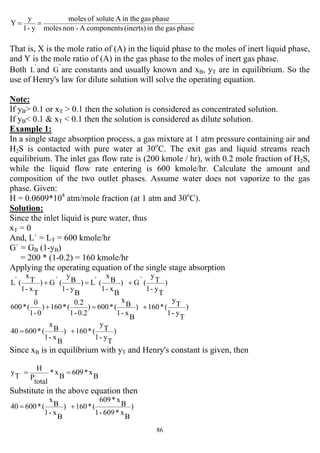
Now plot the operating line by assuming yn+1 to find xn starting from yT to yB, the
following data are obtained:
Step three:
By using the equations of mass flow calculate Gy, Lx for each y, x as shown
64*
y1
y
*`G29*`GGy
−
+=
For example, use y = 0.2, whereas x = 0.00356
Therefore:
0.316464]/0.0929*
0.2-1
0.2
*0.00065329)*(0.000653[yG =+= kg / m2
sec
64*
x1
x
*`L18*`LxL
−
+=
seckg/m8.24164]/0.0929*
0.00356-1
0.00356
*0.04218)*(0.042xL 2
=+=
Step four:
Now we have to calculate a`
yk and a`
xk for each value of Gy, Lx estimated in above
using the following equations:
fractionmole3mkmole/sxL*yG*0.0594a`
yk 0.250.7
=
fractionmole3mkmole/s0.044960.25(8.241)*0.7(0.3164)*0.0594a`
yk ==
Xn Yn+1
0 0.02
0.000332 0.04
0.000855 0.07
0.00207 0.13
0.002631 0.16
0.00356 0.2](https://image.slidesharecdn.com/masstransferdrauroba-150501120755-conversion-gate01/85/Mass-transfer-dr-auroba-121-320.jpg)
![122
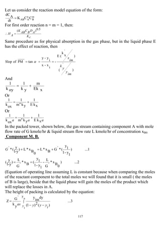
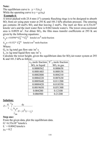
Example 7:
A tower packed with 25.4 mm (1") ceramic Rasching rings is to be designed to absorb
SO2 from air using pure water at 293 K and 101.3 kPa absolute pressure. The entering
gas contains 20 mol% SO2 and that leaving 2 mol%. The inert air flow at 6.53x10⁻⁴
kmole/ air/s and the inert water flow is 0.042 kmole water/s. The tower cross-sectional
area is 0.0929 m2
for dilute SO2 the overall mass transfer coefficient:
k`OG a =16 kmole/hr m3
packing 105
pa
Calculate the tower height on the basis of the overall driving force that is [(NTU)oy,
(HTU)oy], given the equilibrium data for SO2/air-water system at 293 K and 101.3 kPa
as follow:
xA mole fraction
SO2 in liquid
Y*
A mole fraction
SO2 in gas
0.0000562 0.000658
0.0001403 0.000158
0.0002800 0.004210
0.0004220 0.007630
0.0005640 0.011200
0.0008420 0.018550
0.0019650 0.051300
0.0042000 0.121000
0.0069800 0.212000
Solution
∫
−−
=
B
y
)*(2)1(
dy*
my
s`
oyk
`G
Z
T
y yyy
Step one: From the given data, plot the equilibrium data.
G`=6.53x10⁻⁴
kmole/s = 2.3508 kmole/hr
L` = 0.0042 kmole/s
yB = 0.2
yT = 0.02
xT = 0
Make material balance to calculate xB
Ty-1
Ty
)
11
(*
`
`
L
By1
+
−
−
−
=
− Tx
Tx
Bx
Bx
G
By
0.02-1
0.02
)
01
0
1
(*
000653.0
0.042
0.21
2.0
+
−
−
−
=
− Bx
Bx
Then: xB = 0.00355
Step two:](https://image.slidesharecdn.com/masstransferdrauroba-150501120755-conversion-gate01/85/Mass-transfer-dr-auroba-124-320.jpg)


![147
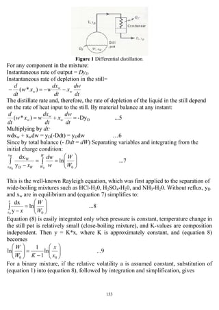
C- RECTIFICATION WITH REFLUX
It is also called fractionation (distillation) or multiple stages with reflux.
On each stage there are liquid and vapor flow counter-currently, mixed and equilibrated on each
stage. Therefore, the liquid and vapor leave the stage are in equilibrium.
The final vapor comes from overhead contains high concentration of the M. V. C., is condensed
and portion of it removed as top product, while the remaining liquid is returned to the top tray of
the column as reflux liquid.
The liquid leaving the bottom, which is less in the M. V. C. or in other words rich of the L. V. C.,
is withdrawn as bottom product, portion of this product is evaporated in the re-boiler and sent back
to the bottom stage (or tray).
The methods of calculation of the number of stages are:
1- McCabe – Thiele Method
In 1925, McCabe and Thiele published an approximate graphical method for combining the
equilibrium with the operating – line curves to estimate, for a given binary feed mixture and
column operating pressure, the number of equilibrium stages and the amount of reflux required for
a desired degree of separation of the feed.
The McCabe – Thiele method determine not only N, the number of equilibrium stages, but also
Nmin, Rmin, and the optimal stage for feed entry. Following the application of the McCabe – Thiele
method, energy balances are applied to estimate condenser and re-boiler heat duties.
Besides the equilibrium curve, the McCabe – Thiele method involve a 45o
reference line, separate
operating lines for the upper rectifying (enriching) section of the column and the lower stripping
(exhausting) section of the column, and a fifth line (the q-line or feed line) for the phase or thermal
condition of the feed. The most important assumptions made to apply this method are:
1- The two components have equal and constant molar enthalpies of vaporization (latent heat).
2- Component sensible enthalpy changes (Cp ∆T) and heat of mixing are negligible compared to
latent heat changes.
3- The column is well insulated so that heat loss is negligible.
4- The pressure is uniform throughout the column (no pressure drop).
These assumptions are referred to as the McCabe – Thiele assumptions leading to the condition of
constant molar flow rate in both sections of the column (rectifying & stripping) or we can say
constant molar flow rate in the tower.
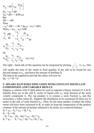
Establishing the operating line equation
Consider the following section in the distillation column
O. M. B. on a certain stage (n):
Vn+1 + Ln-1 = Vn + Ln
[A] M. B. on stage (n):
Vn+1 * yn+1 + Ln-1 * xn-1 = Vn * yn + Ln * xn
Where:
Vn+1: molar vapor flow rate from stage n+1, mol/hr
Ln : molar liquid flow rate from stage n, mol/hr
yn+1: mole fraction of (A) in stream Vn+1
xn: mole fraction of (A) in stream Ln
yn & xn are in equilibrium on tray n with a temperature of Tn.](https://image.slidesharecdn.com/masstransferdrauroba-150501120755-conversion-gate01/85/Mass-transfer-dr-auroba-149-320.jpg)
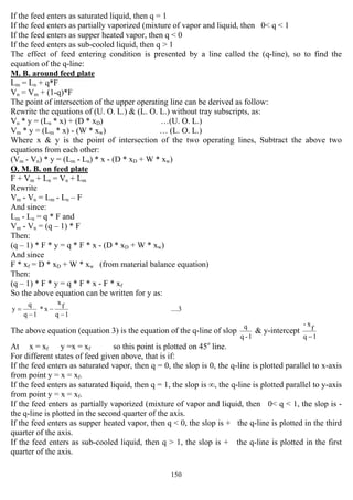
![148
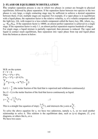
0
0.2
0.4
0.6
0.8
1
0 0.2 0.4 0.6 0.8 1
x
y
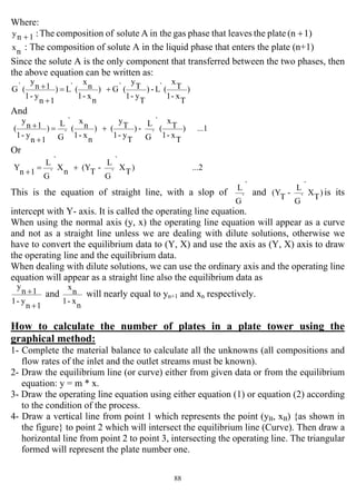
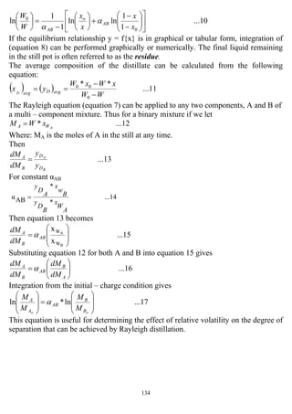
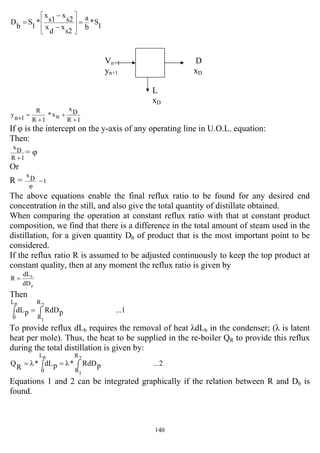
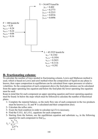
A- Equations for rectification (enriching) section:
O. M. B. for the entire column:
F = D + W
[A] M. B. for the entire column:
F * xf = D * xD + W * xw
O. M. B. around the selected section:
Vn+1 = Ln + D
[A] M. B. for the selected section:
Vn+1 * yn+1= Ln * xn + D * xD
Solving for yn+1
Dx*
1nV
D
nx*
1nV
nL
1ny
+
+
+
=+
Since R= reflux ratio =
D
nL
= constant
Vn+1 = Ln + D
= D * ( R + 1)
Then
....1
1R
Dx
nx*
1R
R
1ny
+
+
+
=+
The above equation (equation 1) is a straight line equation of slop
1R
R
+
& y-intercept
1R
D
x
+
at x=0.
It is called the upper operating line equation (U. O. L.). It intersects the 45o
line at y = x =xD.
The theoretical number of stages is determined by starting from xD and stepping off the first plate
at x1 and so on
Slop of the operating
Line =
1R
R
+](https://image.slidesharecdn.com/masstransferdrauroba-150501120755-conversion-gate01/85/Mass-transfer-dr-auroba-150-320.jpg)
![149
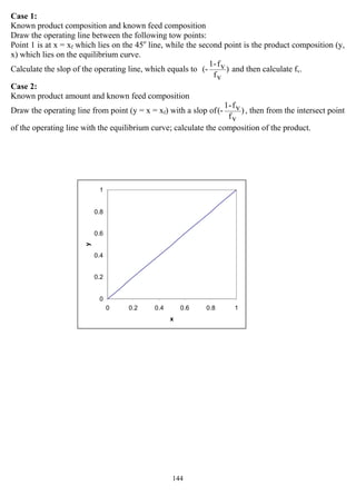
0
0.2
0.4
0.6
0.8
1
0 0.2 0.4 0.6 0.8 1
x
y
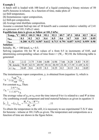
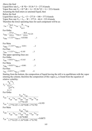
B- Equations for stripping section:
O. M. B. around the selected section (stripping section:
Vm+1 = Lm - W
[A] M. B. for the selected section:
Vm+1 * ym+1= Lm * xm - W * xw
Solving for ym+1
...2Wx*
1mV
W
mx*
1mV
mL
1my
+
−
+
=+
The above equation (equation 2) represents the lower operating line equation (L. O. L.) of slop
1m
V
mL
+
and it intersects the 45o
line (that is y = x) at x = xw. And at x = 0 it intersects the y-axis at
1mV
wx*W
y
+
−=
C- Effect of feed condition:
The condition of feed F entering the tower determines the relation between Vm and Vn also Lm and
Ln, such as partially vaporized feed. So we represent the condition of feed by (q) where:
feedofionvaporizatofheatlatentMolal
conditionenteringatfeedofmoleonevaporizetoneededHeat
q =
So we can define (q) as the fraction of feed that is entered as liquid.
l
HvH
f
HvH
q
−
−
=
Where:
Hv: enthalpy of feed at the dew point (saturated vapor enthalpy).
Hl: enthalpy of feed at the bubble point (saturated liquid enthalpy).
Hf: enthalpy of feed at its entering temperature (entrance conditions).
Therefore;
If the feed enters as saturated vapor, then q = 0](https://image.slidesharecdn.com/masstransferdrauroba-150501120755-conversion-gate01/85/Mass-transfer-dr-auroba-151-320.jpg)
![153
0
0.1
0.2
0.3
0.4
0.5
0.6
0.7
0.8
0.9
1
0 0.2 0.4 0.6 0.8 1
x
y
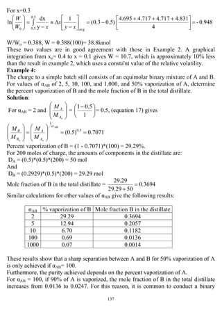
When the two operating lines touch the equilibrium curve, a (Pinch point) at y`, and x` occurs.
Where the number of stages required becomes infinite, so the slop of the U. O. L. is as follow:
`x
D
x
`y
D
x
1
min
R
min
R
−
−
=
+
For vertical q-line (y`, and x`) are substituted by (yf, and xf) as shown in the figure and then the
above equation can be written as
f
x
f
y
f
y
D
x
min −
−
=R
And for horizontal q-line y`, and x`) are substituted by (yf, and xc) as shown in the figure and then
the above equation can be written as
c
x
f
x
f
x
D
x
min −
−
=R
Or can be determined graphically as
shown:
NOTE:
At minimum reflux, it requires minimum
size of condenser & re-boiler.
The number of plates and minimum reflux ratio can be found analytically using Underwood &
Fenske equations:
averagelogα
]W)
Ax
Bx
(*D)
Bx
Ax
log[(
1N =+
For small variation in α
α aaver. = (αD * αw)½
αD: Relative volatility of the overhead product
αw: Relative volatility of the bottom product
While the minimum reflux ratio equation is:
}
f
x1
)
D
xα(1
f
x
D
x
{
1α
1
min
R
−
−
−
−
=](https://image.slidesharecdn.com/masstransferdrauroba-150501120755-conversion-gate01/85/Mass-transfer-dr-auroba-155-320.jpg)
![156
0
0.1
0.2
0.3
0.4
0.5
0.6
0.7
0.8
0.9
1
0 0.2 0.4 0.6 0.8 1
x
y
2- Enriching tower:
This process is used for mixtures lean in M. V. C.
Feed is introduced from the bottom of the column as saturated vapor or superheated vapor, where
no re-boiler is used. The composition of bottom product is comparable to feed composition
(slightly less than xf).
O. M. B. on the top of the column
Vn+1 = Ln + D
[A] M. B. on the bottom of the column
yn+1 * Vn+1 = xn * Ln + xD * D
The operating line equation is:
1nV
Dx*D
nx*
1nV
L
1ny
+
+
+
=+
n
Vn = F if the feed is saturated vapor
And Vn = (1-q) * F if the feed is superheated vapor
3- Rectification with direct steam injection:
In this type of processes the heat is supplied to the bottom of the tower by direct steam injection,
where the re-boiler is not needed.
O. M. B. on the column
F + S = D + W
[A] M. B.
F * xf = D * xD + W * xW
The enriching section is not affected, because no change done but for the stripping section, the
material balance will be:
O. M. B.
Lm + S = Vm+1 + W
[A] M. B.
Lm * xm = Vm+1 * ym+1 + W * xW](https://image.slidesharecdn.com/masstransferdrauroba-150501120755-conversion-gate01/85/Mass-transfer-dr-auroba-158-320.jpg)
![158
Vs+1 = Vn+1 = Ln + D
Vn+1 = Ln + D
[A] M. B.
ys+1 * Vs+1 = xs * Ls + xD * D + xZ * Z
Rewrite for y and substitute Vs+1 by Vn+1, so
1nV
Z
x*ZDx*D
Sx*
1n
V
S
L
1Sy
+
+
+
+
=+
DLn
Z
x*ZDx*D
Sx*
D
n
L
Z
n
L
1Sy
+
+
+
+
−
=+
D
nL
R =Θ
1R
Z
x*D
Z
D
x
S
x*
1R
D
ZR
1S
y
+
+
+
+
−
=
+
∴
The above equation is the operating line equation for the side stream of slop
1R
D
ZR
+
−
(
1n
V
S
L
+
) and
intersect the y-axis at y =
1R
Z
x*D
Z
D
x
+
+
(
1nV
Z
x*ZDx*D
+
+
). So to calculate the number of plates
using the McCabe-Thiele method, follow the steps:
1- Complete the M. B., so the mole fraction of all streams must be known.
2- Plot the equilibrium data and locate xD, xZ, xf, xW on the 45o
line.
3- Plot the U. O. L. using the points, (y = x = xD), (y =
1R
D
x
+
, x =0).
4- Plot the side stream q-line which has a slop = ∞ (saturated liquid), from the point y =x =xZ.
5- Plot the side stream operating line between the points; the intersection of the U.O.L. & the side
stream q-line and the (y =
1R
Z
x*D
Z
D
x
+
+
, x =0), with slop
1R
D
ZR
+
−
.
6- Plot the q-line of the feed from the point y =x = xf as before (depending on the feed condition).
7- From the point of intersection of the side stream operating line and the q-line of the feed draw
the L.O.L. to intersect the 45o
line at y =x = xw.
8- Step –off the stages as before.
Then the theoretical number of plates = N-1
As shown in below](https://image.slidesharecdn.com/masstransferdrauroba-150501120755-conversion-gate01/85/Mass-transfer-dr-auroba-160-320.jpg)
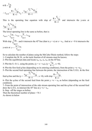
![165
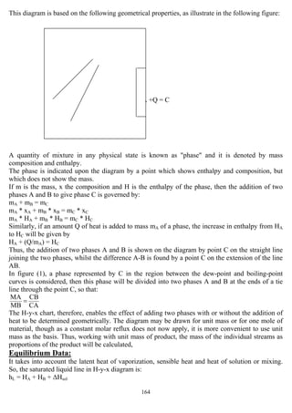
hL = xA * CpA * (T-Tref) + (1- xA) * CpB * (T-Tref) + ∆Hsol
HV = hL * λmix
Where:
λmix = xA * λA + (1-xA) * λB
Properties and uses of enthalpy – concentration chart
Lever – arm rule:-
Let the streams S1 and S2 of composition Z1 & Z2 respectively mixed adiabatically to give another
mixture S3 of composition Z3, so the material balance and energy balances will be:
O. M. B.
S1 + S2 = S3 …1
[M.V.C.] M. B.
S1 * Z1 + S2 * Z2 = S3 * Z3 …2
[M.V.C.] E. B.
S1 * H1 + S2 * H2 = S3 * H3 …3
From equations (1, 2)
13
32
2
1
ZZ
ZZ
S
S
−
−
=
And from equations (1, 3)
13
32
2
1
Hh
HH
S
S
−
−
=
CA
CB
S
S
2
1
= hL & HV
kJ/kg
(kJ/kmole)
xA & yA
h
yA
Z
xA
The tie (ab) represents the enthalpy
For non – adiabatic mixing which is similar to that for adiabatic but with addition of Q (Q is heat
of mixing or heat losses or the net), so
S1 * H1 + S2 * H2 = S3 * H3 + Q](https://image.slidesharecdn.com/masstransferdrauroba-150501120755-conversion-gate01/85/Mass-transfer-dr-auroba-167-320.jpg)

![167
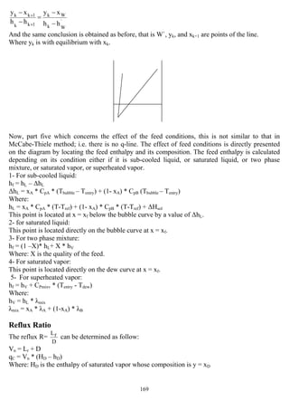
Overall column M.B.
F = D + W …1
[M.V.C.] M. B.
F * xf = D * xD + W * xw …2
[M.V.C.] E. B.
F * hf + qr = qc + D * hD + W * hw …3
Then:
)
W
rq
W
(h*W)
D
cq
D
(h*D
f
h*F −++=
Let Qc =
D
cq
(heat lost by condenser per kgm of distillate)
And Qr =
W
rq
(heat gained by re-boiler per kgm of residue)
Then:
...4`
W
h*W`
D
h*D
f
h*F +=
Where:
`
D
h =
cQ
D
h +
`
W
h =
rQ
W
h −
Substitute equation 1 into 2 and 4, then
(D + W) * xf = D * xD + W * xw
D * (xD – xf) = W * (xW – xf) …5
`
W
h*W`
D
h*D
f
h*W)(D +=+
...6)`
W
h-
f
(h*W)
f
h-`
D
(h*D =
Dived equation 5 by 6
`
W
h
f
h
W
x
f
x
f
h`
D
h
f
x
D
x
−
−
=
−
−
This equation states that `
D
h , hf and `
W
h is on a straight line at the points D`, f, and W`
Where:
D`: is the pole point of all operating lines above feed.
W`: is the pole point of all operating lines below feed.
f: is the feed point.](https://image.slidesharecdn.com/masstransferdrauroba-150501120755-conversion-gate01/85/Mass-transfer-dr-auroba-169-320.jpg)
![168
Part three:
Operating lines above the feed:
Total M. B.
Vn = Ln+1 + D …1
[M.V.C.] M. B.
Vn * yn = Ln+1 * xn+1 + D * xD …2
Enthalpy M. B.
Vn * hn = Ln+1 * hn+1 + D * (hD + Qc)
Or
Vn * hn = Ln+1 * hn+1 + D * ( `
D
h ) …3
Substitute equation (1) into (2) and (3)
(D + Ln+1) * yn = Ln+1 * x n+1 + D * xD
D * (xD – yn) = Ln+1 * (yn – x n+1) …4
`h*Dh*Lh*)L(D D1n1nn1n
+=+ +++
...5)hh(*L)nh`(h*D 1nn1nD ++
−=−
Dived equation 4 by 5
1n
hnh
1n
xny
nh`
D
h
ny
D
x
+
−
+
−
=
−
−
Which is also as before an equation of straight line, which states that D`, yn, and xn+1 are points of
the line.
xn+1 is with equilibrium with yn+1
Part Four
Operating lines below the feed:
Total M. B.
Lk+1 = Vk + W
Vk = Lk+1 - W …1
[M.V.C.] M. B.
Vk * yk = Lk+1 * xk+1 - W * xW …2
Enthalpy M. B.
Vk * hk = Lk+1 * hk+1 - W * (hW - Qr)
Or
Vk * hk = Lk+1 * hk+1 - W * ( `
W
h ) …3
Substitute equation (1) into (2) and (3), and by using the same procedure as done in before, then:](https://image.slidesharecdn.com/masstransferdrauroba-150501120755-conversion-gate01/85/Mass-transfer-dr-auroba-170-320.jpg)

![174
Also
B
k
A
k
AB
α =∴
Hence:
B
x
A
x
*
AB
α
B
y
A
y
=
The same is done for each component, then substitute in equation 2 to get:
B
y
1
B
x
D
x
*
DB
α
B
x
C
x
*
CB
α
B
x
B
x
*
BB
α
B
x
A
x
*
AB
α =+++
Or
B
y
1
B
x
in
1n
x*α
=
∑
=
=
Or
∑
=
=
=
in
1n
x*α
B
y
B
x
Substitute in equation 2, then:
...3
in
1n
x*α
A
x*
AB
α
A
y
∑
=
=
=
...4
in
1n
x*α
C
x*
CB
α
C
y
∑
=
=
=
...5
in
1n
x*α
D
x*
DB
α
D
y
∑
=
=
=
Equations 3, 4, and 5 are the equilibrium equations.
Calculations of bubble point and dew point
Vapor pressure of a liquid at certain temperature and total pressure can be found from Henry's law.
A
x*0
A
P
A
P = Also
T
P*
A
y
A
P =
And
A
x*H
A
P = where: H is Henry's constant
A
x*
A
k
T
P
A
x*H
T
P
A
P
y ===
So the partial pressure for component A is given as:
PA= PT * kA * xA
Then at bubble point the total vapor pressure = P * (Σ k * x) = PT
If any inert gas present, then:
Pinert = PT * [1- (Σ k * x)]](https://image.slidesharecdn.com/masstransferdrauroba-150501120755-conversion-gate01/85/Mass-transfer-dr-auroba-176-320.jpg)

![181
6- Substitute ymi in the L.O.L equation and find x(m+1)i for each component.
7- Repeat steps 6 & 7 until you reach xmi > xfi then substitute ymi obtained from the equilibrium
equation in the U.O.L. equation for each component to find xmi and repeat the same
procedure as done in steps 6 &7 until you reach xni = xDi. Step off the number of plates
required (N).
Theoretical number of plates = N -1
Minimum reflux ratio
The method used for determine the minimum reflux ratio for binary mixture graphically can not be
used when we deal with multi-component system, as we can not draw an equilibrium curve for this
system. There are two methods for determining the minimum reflux:
1- Colburn's Method:-
The following equation was proposed by Colburn to calculate the minimum reflux ratio:
]
x
x
*-
x
x
[R
nH
DH
LH
nL
DL
1
LH
min α
α
1
−
=
Where:
αDL: The relative volatility of L.K. component to the H.K. component.
xDL: The mole composition of the L.K. component in the distillate.
xDH: The mole composition of the H.K. component in the distillate.
XnL: The mole composition of the L.K. component in the pinch point.
XnH: The mole composition of the H.K. component in the pinch point.
Where:
)1)(r(1 fh
f
nL xαf
r
x
∑++
=
f
r
nL
x
xnH =
For rf: is the estimated ratio of the key components on the feed plate.
For a liquid feed at its bubble point, rf equals to the ratio of the key components in the feed.
nH
x
nL
x
f
r =
Otherwise rf is calculated as the ratio of the key component in liquid part of the feed.
xfh: is the mole fraction of each component in liquid portion of feed heavier than heavy key in feed.
α: relative volatility of the components relative to the H.K.
2- Underwood's Method
For conditions where the relative volatilities remain constant, Underwood has developed the
following equations from which Rmin may be calculated:
q1.....
θα
x*α
θα
x*α
θα
x*α
C
fCC
B
fBB
A
fAA
−=+
−
+
−
+
−
And
1R.....
θα
x*α
θα
x*α
θα
x*α
min
C
DCC
B
DBB
A
DAA
+=+
−
+
−
+
−
Where:](https://image.slidesharecdn.com/masstransferdrauroba-150501120755-conversion-gate01/85/Mass-transfer-dr-auroba-183-320.jpg)
![182
xfA, xfB, xfC, xDA, xDB, xDC …etc are the mole fraction of components A,B,C, …etc in the feed and
distillate, A being the light key and B is the heavy key.
αA, αB, αC, are the relative volatilities of components with respect to the heavy key.
q: is the heat required to vaporize one mole of feed to the molar latent heat of the feed.
θ: is the root of the first equation where:
αH < θ < αL
Number of minimum number of plates:
Using Fensk's equation
avLH
BLHDHL
min
)log(α
])/x(x*)/xlog[(x
1N =+
Where:
(αLH)av = [(αLH)f * ( αLH))B * (αLH)D]1/3
Relation between reflux ratio and number of plates:
The Gilliland's correlation related the reflux ratio R and the number N of plates, in which only the
minimum reflux ratio Rmim and the number of plates at total reflux (i.e. Nmin) are required. This is
shown in the following equation, where (R-Rmin)/(R+1) is plotted against the group [(N+1) –
(Nmin+1)]/(N+2), (the first one represent y-axis while the second one the x-axis). The relation can
be given as follow:
]
x
1.805
x*0.315exp[1.491
2N
NN
y 0.1
min
−+−=
+
−
= Where
1
min
+
−
=
R
RR
x
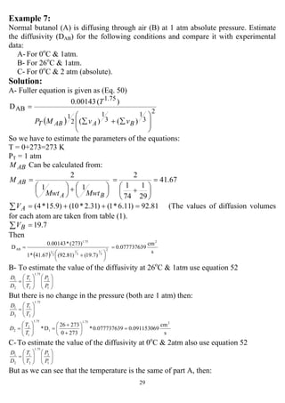
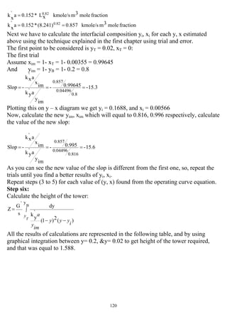
Example 10:
Suppose a mixture of hexane, Heptane and Octane to be separate to give products as shown in the
table. What will be the value of the minimum reflux ratio, if the feed is liquid at its boiling point?
Then find the minimum number of plates required. Investigate the change in N with R and find the
number of plates if R=10. (Plot N vs. R).
Component F mole xf D mole xD W mole xW Relative volatility
Hexane 40 0.4 40 0.534 0 0 2.7
Heptane 35 0.35 34 0.453 1 0.04 2.22
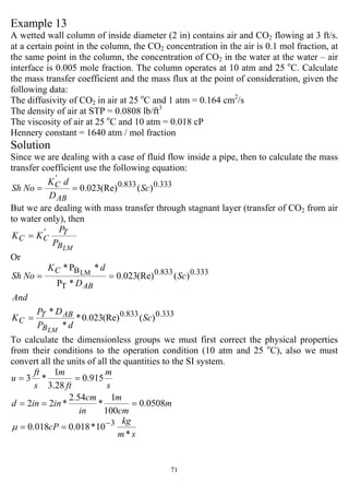
Octane 25 0.25 1 0.013 24 0.96 1.0](https://image.slidesharecdn.com/masstransferdrauroba-150501120755-conversion-gate01/85/Mass-transfer-dr-auroba-184-320.jpg)
![183
Solution
The L.K. is Heptane, H.K. is Octane
Then αHO = 2.7, αHeoO = 2.2, αOO = 1.0
Using Underwood's method:
q1.....
θα
x*α
θα
x*α
θα
x*α
C
fCC
B
fBB
A
fAA
−=+
−
+
−
+
−
Where q = 1 (saturated liquid), then
0
θ1
0.25*1
θ2.22
0.35*2.22
θ2.7
0.4*2.7
=
−
+
−
+
−
αH < θ < αL or 1< θ < 2.22
The above equation is solved by trail and error, so assume θ = 1.15
0.243
θα
x*α f
−=
−
∴∑
Assume θ = 1.17, then
00.024
θα
x*α f
≈−=
−
∴∑ This is acceptable value
Now substitute the value of θ in the following equation
1R.....
θα
x*α
θα
x*α
θα
x*α
min
C
DCC
B
DBB
A
DAA
+=+
−
+
−
+
−
1R
1.171
0.013*1
1.172.22
0.453*2.22
1.172.7
0.534*2.7
min +=
−
+
−
+
−
Rmin = 0.827
The minimum number of plates Nmin can be calculated by:
avLH
BLHDHL
min
)log(α
])/x(x*)/xlog[(x
1N =+
Here consider αLH is constant for F, D and W, then
av
min
log(2.22)
)](0.96/0.04*/0.013)log[(0.453
1N =+
Nmin +1 = 8.5
Nmin = 7.5
Now to find the effect of R on the number of plates use the equation:
]
x
1.805
x*0.315exp[1.491
2N
NN
y 0.1
min
−+−=
+
−
= ..* Where
1
min
+
−
=
R
RR
x
Establish a table as shown in below by assuming R starting from Rmin to a value of 10 for each
value find x for each R and then substitute in equation (*) and find y then evaluate N.
Finally plot N vs. R as given in below:
Θ Rmin = 0.827 ≈0.83
And Nmin = 7.5
Value of R
1
min
+
−
=
R
RR
x ]
x
1.805
x*0.315exp[1.491y 0.1
−+−=
y-1
Ny*2
N min+
=
1 0.085 0.547 18.97≈19
2 0.39 0.31 11.77 ≈12
5 0.695 0.1504 9.18 ≈10
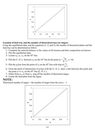
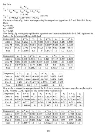
10 0.833 0.0823 8.35 ≈ 9](https://image.slidesharecdn.com/masstransferdrauroba-150501120755-conversion-gate01/85/Mass-transfer-dr-auroba-185-320.jpg)
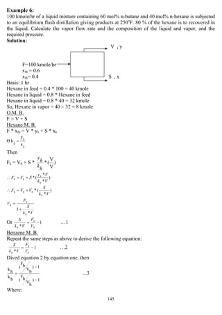
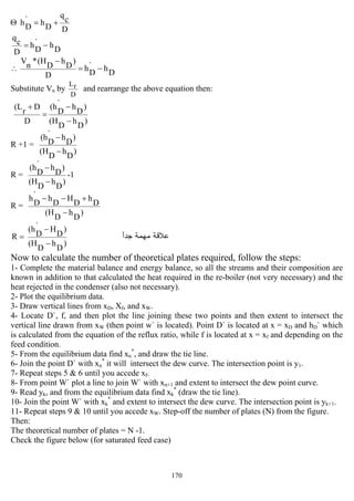
![184
5
9
13
17
21
0 3 6 9 12
R
N
Example 11:
A mixture of Ortho, Meta and Para mono-nitro-toluene containing 60, 4 and 36 mol% respectively
of the three isomers is to be continuously distilled to give a top product of 98 mol% Ortho, the
bottom product is to contain 12.5 mol% Ortho. The mixture is to be distilled at a temperature of
410 K requiring a pressure in the boiler of about 6 kN/m2
(0.06 bar). If a reflux ratio of 5 is used,
how many theoretical plates will be required and what will be the approximate composition of the
top product stream? Given the following data:
αOP = 1.7
Both at a range of 380 to 415 K
αMP = 1.16
Solution:
As a first estimation, suppose the distillate to contain 0.6 mol% Meta and 1.4 mol% Para. Then by
material balance find the composition of the bottom.
Basis 100 kmole of feed
D is the top product with composition of xDO (mole fraction of Ortho).
W is the bottom product with composition of xWO (mole fraction of Ortho).
O. M. B.
F = D + W
[Ortho] O. M. B.
60 = D * xDO + W * xWO
60 = (100-W) * 0.98 + 0.125 * W
Then D = 55.56 kmole and W = 44.44 kmole
The M. B. will give the compositions and amounts of all streams as shown in the following table:
Feed Distilled Bottom
Component
kmole Mol% kmole Mol% kmole Mol%
Ortho (O) 60 60 54.44 98 5.56 12.5
Para (P) 36 36 0.79 0.6 35.21 79.2
Meta (M) 4 4 0.33 1.4 3.67 8.3
Now find the operating lines equations for each component:](https://image.slidesharecdn.com/masstransferdrauroba-150501120755-conversion-gate01/85/Mass-transfer-dr-auroba-186-320.jpg)
![187
Component x13 α * x13 y13 x14 α * x14 y14 x15 α * x15 y15
Ortho o 0.911 1.5487 0.943 0.936 1.5912 0.959 0.955 1.6235 0.972
Meta M 0.025 0.029 0.018 0.02 0.0232 0.014 0.015 0.01755 0.01
Para P 0.064 0.064 0.039 0.044 0.044 0.027 0.03 0.03 0.018
sum 1.0 1.6417 1.0 1.0 1.6584 1.0 1.0 1.67105 1.0
Component x16 α * x16 y16 x17
Ortho o 0.971 1.6507 0.983 0.983
Meta M 0.01 0.0116 0.007 0.007
Para P 0.019 0.019 0.01 0.01
sum 1.0 1.6813 1.0 1.0
And that is the end of calculation because the composition of the product D exceed the given value
(0.98)
Therefore the final approximate composition is:
Ortho: 0.983
Meta: 0.007
Para: 0.01
And the theoretical number of plates required = 17 - 1 = 16 plates
Example 12(stage by stage method)
A mixture of benzene and toluene containing 40 mole% of benzene is to be separated to give a
product of 90 mole % of benzene at the top, and a bottom product with not more than 10 mole% of
benzene. The feed is heated so that it enters the column at its boiling point, and the vapor leaving
the column is condensed but not cooled, and provides reflux and product. It is proposed to operate
the unit with reflux ratio of 3 kmol / kmol product. It is required to find the number of theoretical
plates needed and the position of entry of the feed. The equilibrium data are given in the table
below:
Solution:
Basis 100 kmole of feed
A total material balance gives:
100 = D + W
[Benzene M. B.]
100 * 0.4 = 0.9 * D + 0.1 * W
Thus:
40 = 0.9 * (100- W) + 0.1 * W
Whence:
W = 62.5 kmole and D = 37.5 kmole
D
L
R n
=
Ln = 3 * D = 112.5
And
Vn = Ln + D = 150
xBenzene 0 0.1 0.2 0.3 0.4 0.5 0.6 0.7 0.8 0.9 1.0
yBenzene 0 0.2 0.38 0.51 0.63 0.71 0.78 0.85 0.91 0.96 1.0](https://image.slidesharecdn.com/masstransferdrauroba-150501120755-conversion-gate01/85/Mass-transfer-dr-auroba-189-320.jpg)


![r [Autosaved].pptx](https://cdn.slidesharecdn.com/ss_thumbnails/module5-masstransferautosaved-221221175506-163cc248-thumbnail.jpg?width=640&height=640&fit=bounds)


![5G Explained! A High Level Overview [Introduction]](https://cdn.slidesharecdn.com/ss_thumbnails/5gexplainedahighleveloverview-260119165306-cc137a3e-thumbnail.jpg?width=640&height=640&fit=bounds)


