This document discusses inner product spaces and how inner products can be defined on vector spaces to generalize concepts like the dot product, vector norms, angles between vectors, and distances between vectors. It provides examples of defining inner products on spaces like Rn, the space of polynomials Pn, and the space of 2x2 matrices M22. It shows how norms, orthogonality, and distances can be calculated in these spaces based on their defined inner products. The document also discusses how different inner products can lead to different geometries beyond standard Euclidean geometry.

1. Chapter 7
Inner Product Spaces
大葉大學 資訊工程系
鈴玲黃
Linear Algebra

2. Ch7_2
Inner Product Spaces
In this chapter, we extend those concepts of Rn
such as:
dot product of two vectors, norm of a vector, angle between
vectors, and distance between points, to general vector space.
This will enable us to talk about the magnitudes of functions
and orthogonal functions. This concepts are used to
approximate functions by polynomials – a technique that is
used to implement functions on calculators and computers.
We will no longer be restricted to Euclidean Geometry,
we will be able to create our own geometries on Rn
.

3. Ch7_3
7.1 Inner Product Spaces
The dot product was a key concept on Rn
that led to definitions of norm,
angle, and distance. Our approach will be to generalize the dot product of
Rn
to a general vector space with a mathematical structure called an inner
product. This in turn will be used to define norm, angle, and distance for
a general vector space.

4. Ch7_4
Definition
An inner product on a real spaces V is a function that associates a
number, denoted 〈 u, v 〉 , with each pair of vectors u and v of V.
This function has to satisfy the following conditions for vectors u, v,
and w, and scalar c.
1. 〈 u, v 〉 = 〈 v, u 〉 (symmetry axiom)
2. 〈 u + v, w 〉 = 〈 u, w 〉 + 〈 v, w 〉 (additive axiom)
3. 〈 cu, v 〉 = c 〈 u, v 〉 (homogeneity axiom)
4. 〈 u, u 〉 0, and 〈 u, u 〉 = 0 if and only if u = 0
(position definite axiom)
A vector space V on which an inner product is defined is called an
inner product space.
Any function on a vector space that satisfies the axioms of an inner product
defines an inner product on the space.
There can be many inner products on a given vector space.

5. Ch7_5
Example 1
Let u = (x1, x2), v = (y1, y2), and w = (z1, z2) be arbitrary vectors in
R2
. Prove that 〈 u, v 〉 , defined as follows, is an inner product
on R2
.
〈 u, v 〉 = x1y1 + 4x2y2
Determine the inner product of the vectors (−2, 5), (3, 1) under
this inner product.
Solution
Axiom 1: 〈 u, v 〉 = x1y1 + 4x2y2 = y1x1 + 4y2x2 = 〈 v, u 〉
Axiom 2: 〈 u + v, w 〉 = 〈 (x1, x2) + (y1, y2) , (z1, z2) 〉
= 〈 (x1 + y1, x2 + y2), (z1, z2) 〉
= (x1 + y1) z1 + 4(x2 + y2)z2
= x1z1 + 4x2z2 + y1 z1 + 4 y2z2
= 〈 (x1, x2), (z1, z2) 〉 + 〈 (y1, y2), (z1, z2) 〉

6. Ch7_6
Axiom 3: 〈 cu, v 〉 = 〈 c(x1, x2), (y1, y2) 〉
= 〈 (cx1, cx2), (y1, y2) 〉
= cx1y1 + 4cx2y2 = c(x1y1 + 4x2y2)
= c 〈 u, v 〉
Axiom 4: 〈 u, u 〉 = 〈 (x1, x2), (x1, x2) 〉 = 04 2
2
2
1 ≥+ xx
Further, if and only if x1 = 0 and x2 = 0. That is u =
0. Thus 〈 u, u 〉 0, and 〈 u, u 〉 = 0 if and only if u = 0.
The four inner product axioms are satisfied,
〈 u, v 〉 = x1y1 + 4x2y2 is an inner product on R2
.
04 2
2
2
1 =+ xx
The inner product of the vectors (−2, 5), (3, 1) is
〈 (−2, 5), (3, 1) 〉 = (−2 × 3) + 4(5 × 1) = 14

7. Ch7_7
Example 2
Consider the vector space M22 of 2 × 2 matrices. Let u and v
defined as follows be arbitrary 2 × 2 matrices.
Prove that the following function is an inner product on M22.
〈 u, v 〉 = ae + bf + cg + dh
Determine the inner product of the matrices .




















==
hg
fe
dc
ba
vu ,
Solution
Axiom 1: 〈 u, v 〉 = ae + bf + cg + dh = ea + fb + gc + hd = 〈 v,
u 〉
Axiom 3: Let k be a scalar. Then
〈 ku, v 〉 = kae + kbf + kcg + kdh = k(ae + bf + cg + dh) = k 〈 u,
v 〉 4)01()90()23()52(,
09
25
10
32
=×+×+×−+×=






 −











 −
09
25
and
10
32

8. Ch7_8
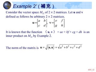
Example 3
Consider the vector space Pn of polynomials of degree ≤ n. Let f
and g be elements of Pn. Prove that the following function
defines an inner product of Pn.
Determine the inner product of polynomials
f(x) = x2
+ 2x – 1 and g(x) = 4x + 1
∫=
1
0
)()(g, dxxgxff
Solution
Axiom 1: fgdxxfxgdxxgxfgf ,)()()()(,
1
0
1
0
=== ∫∫
hghf
dxxhxgdxxhxf
dxxhxgxhxf
dxxhxgxfhgf
,,
)()()]()([
)]()()()([
)()]()([,
1
0
1
0
1
0
1
0
+=
+=
+=
+=+
∫∫
∫
∫Axiom 2:

9. Ch7_9
We now find the inner product of the functions f(x) = x2
+ 2x – 1
and g(x) = 4x + 1
2
)1294(
)14)(12(14,12
1
0
23
1
0
22
=
−−+=
+−+=+−+
∫
∫
dxxxx
dxxxxxxx

10. Ch7_10
Norm of a Vector
Definition
Let V be an inner product space. The norm of a vector v is
denoted ||v|| and it defined by
vv,v =
The norm of a vector in Rn
can be expressed in terms of the dot
product as follows
),,,(),,,(
)(),,,(
2121
22
121
nn
nn
xxxxxx
xxxxx


⋅=
++=
Generalize this definition:
The norms in general vector space do not necessary have geometric
interpretations, but are often important in numerical work.

11. Ch7_11
Example 4
Consider the vector space Pn of polynomials with inner product
The norm of the function f generated by this inner product is
Determine the norm of the function f(x) = 5x2
+ 1.
∫=
1
0
)()(, dxxgxfgf
∫==
1
0
2
)]([, dxxffff
Solution Using the above definition of norm, we get
3
28
1
0
24
1
0
222
]11025[
]15[15
=
++=
+=+
∫
∫
dxxx
dxxx
The norm of the function f(x) = 5x2
+ 1 is .
3
28

12. Ch7_12
Example 2’ ( 補充 )
Consider the vector space M22 of 2 × 2 matrices. Let u and v
defined as follows be arbitrary 2 × 2 matrices.
It is known that the function 〈 u, v 〉 = ae + bf + cg + dh is an
inner product on M22 by Example 2.
The norm of the matrix is




















==
hg
fe
dc
ba
vu ,
2222
, dcba +++== uuu

13. Ch7_13
Definition
Let V be an inner product space. The angle θ between two
nonzero vectors u and v in V is given by
vu
vu,
=θcos
The dot product in Rn
was used to define angle between vectors.
The angle θ between vectors u and v in Rn
is defined by
vu
vu⋅
=θcos
Angle between two vectors

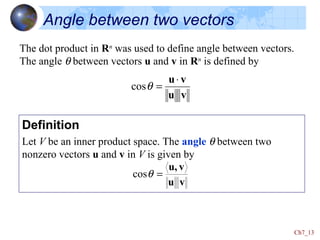
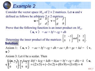
14. Ch7_14
Example 5
Consider the inner product space Pn of polynomials with inner
product
The angle between two nonzero functions f and g is given by
Determine the cosine of the angle between the functions
f(x) = 5x2
and g(x) = 3x
∫=
1
0
)()(, dxxgxfgf
gf
dxxgxf
gf
gf )()(,
cos
1
0∫==θ
Solution We first compute ||f || and ||g||.
3]3[3and5]5[5
1
0
2
1
0
222
==== ∫∫ dxxxdxxx
Thus
4
15
35
)3)(5()()(
cos
1
0
2
1
0
===
∫∫ dxxx
gf
dxxgxf
θ

15. Ch7_15
Example 2” ( 補充 )
Consider the vector space M22 of 2 × 2 matrices. Let u and v
defined as follows be arbitrary 2 × 2 matrices.
It is known that the function 〈 u, v 〉 = ae + bf + cg + dh is an
inner product on M22 by Example 2.
The norm of the matrix is
The angle between u and v is




















==
hg
fe
dc
ba
vu ,
2222
, dcba +++== uuu
22222222
,
cos
hgfedcba
dhcgbfae
++++++
+++
==
vu
vu
θ

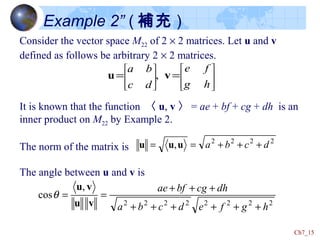
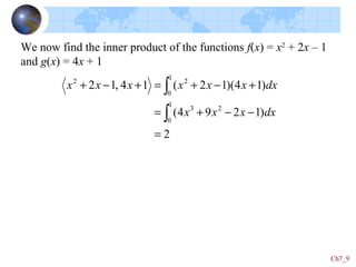
16. Ch7_16
Orthogonal Vectors
Def. Let V be an inner product space. Two nonzero vectors u and
v in V are said to be orthogonal if
0, =vu
Example 6
Show that the functions f(x) = 3x – 2 and g(x) = x are orthogonal
in Pn with inner product
.)()(,
1
0∫= dxxgxfgf
Solution
0][))(23(,23 1
0
23
1
0
=−=−=− ∫ xxdxxxxx
Thus the functions f and g are orthogonal in this inner product
Space.

17. Ch7_17
Distance
Definition
Let V be an inner product space with vector norm defined by
The distance between two vectors (points) u and v is defined
d(u,v) and is defined by
vv,v =
),(),( vuvuvuvu −−=−=d
As for norm, the concept of distance will not have direct
geometrical interpretation. It is however, useful in numerical
mathematics to be able to discuss how far apart various
functions are.

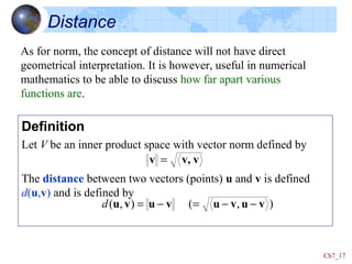
18. Ch7_18
Example 7
Consider the inner product space Pn of polynomials discussed
earlier. Determine which of the functions g(x) = x2
– 3x + 5 or h(x)
= x2
+ 4 is closed to f(x) = x2
.
Solution
13)53(53,53,)],([
1
0
22
=−=−−=−−= ∫ dxxxxgfgfgfd
16)4(4,4,)],([
1
0
22
=−=−−=−−= ∫ dxhfhfhfd
Thus
The distance between f and h is 4, as we might suspect, g is closer
than h to f.
.4),(and13),( == hfdgfd

19. Ch7_19
Inner Product on Cn
For a complex vector space, the first axiom of inner product is
modified to read . An inner product can then be
used to define norm, orthogonality, and distance, as far a real
vector space.
Let u = (x1, …, xn) and v = (y1, …, yn) be element of Cn
. The most
useful inner product for Cn
is
uvvu ,, =
nn yxyx ++= 11vu,
vuvu
u
vuvu
−=
+=
=⊥
),(
0,if
11
d
xxxx nn
※
※
※

⇒

20. Ch7_20
Example 8
Consider the vectors u = (2 + 3i, −1 + 5i), v = (1 + i, − i) in C2
.
Compute
(a) 〈 u, v 〉 , and show that u and v are orthogonal.
(b) ||u|| and ||v||
(c) d(u, v)
Solution
.orthogonalareandthus
055))(51()1)(32(,)(
vu
vu =−−+=+−+−+= iiiiiia
3))(()1)(1(
392613)51)(51()32)(32()(
=−+−+=
=+=−−+−+−+=
iiii
iiiib
v
u
42375)61)(61()21)(21(
)61,21(
),1()51,32(),()(
=+=−−+−+−+=
+−+=
−+−+−+=−=
iiiu
ii
iiiidc vuvu

21. Ch7_21
Homework
Exercise 7.1:
1, 4, 8(a), 9(a), 10, 12, 13, 15, 17(a), 19,
20(a)

22. Ch7_22
7.2 Non-Euclidean Geometry and
Special Relativity
Different inner products on Rn
lead to different measures of
vector norm, angle, and distance – that is, to different geometries.
dot product ⇒ Euclidean geometry
other inner products ⇒ non-Euclidean geometries
Example
Let u = (x1, x2), v = (y1, y2) be arbitrary vectors in R2
. It is proved
that 〈 u, v 〉 , defined as follows, is an inner product on R2
.
〈 u, v 〉 = x1y1 + 4x2y2
The inner product differs from the dot product in the appearance
of a 4. Consider the vector (0, 1) in this space. The norm of this
vector is

23. Ch7_23
2)11(4)00()1,0(),1,0()1,0( =×+×==
Figure 7.1
The norm of this vector in Euclidean geometry is 1;
in our new geometry, however, the norm is 2.

24. Ch7_24
Consider the vectors (1, 1) and (−4, 1). The inner product of these
vectors is
0)11(4)41()1,4(),1,1( =×+−×=−
Figure 7.2
Thus these two vectors are orthogonal.

25. Ch7_25
Let us use the definition of distance based on this inner product to
compute the distance between the points(1, 0) and (0, 1). We
have that
5)11(4)11()1,1(),1,1(
)1,1()1,0()0,1())1,0(),0,1((
=×−+×=−−=
−=−=d
Figure 7.3

26. Ch7_26
7.4 Least-Squares Curves
To find a polynomial that best fits given data points.
Ax = y :
(1) if n equations, n variables, and A−1
exists
⇒ x = A−1
y
(2) if n equations, m variables with n > m
⇒ overdetermined
How to solve it?
We will introduce a matrix called the pseudoinverse of A,
denoted pinv(A), that leads to a least-squares solution
x = pinv(A)y for an overdetermined system.

27. Ch7_27
Definition
Let A be a matrix. The matrix (At
A)−1
At
is called the
pseudoinverse of A and is denoted pinv(A).
Example 1 Find the pseudoinverse of A = .
42
31
21










−
Solution










=











= −
−
297
76
42
31
21
432
211
AAt






−
−
==−
67
729
125
1
)(adj
1
)( 1
AA
AA
AA t
t
t





 −
=




 −






−
−
== −
251
6103
25
1
432
211
67
729
125
1
)()(pinv 1 tt
AAAA

28. Ch7_28
Ax = y x = pinv(A)y
system least-squares solution
If the system Ax=y has a unique solution, the least-squares
solution is that unique solution.
If the system is overdetermined, the least-squares solution is the
closest we can get to a true solution.
The system cannot have many solutions.
Let Ax = y be a system of n linear equations in m variables with
n > m, where A is of rank m.
Ax=y ⇒ At
Ax=At
y ⇒ x = (At
A)−1
At
y
At
A is invertible

29. Ch7_29
Example 2
Find the least-squares solution of the following overdetermined
system of equations. Sketch the solution.
Solution
932
3
6
=+
=+−
=+
yx
yx
yx
The matrix of coefficients is








=








= −
9
3
6
32
11
11
and yA






=











= −
−
116
66
32
11
11
311
211
AAt






==−
116
66
30
1
)(adj
1
)( 1
AA
AA
AA t
t
t





 −
=




 −






−
−
== −
6120
4175
30
1
311
211
66
611
30
1
)()(pinv 1 tt
AAAA
rank(A)=2 ⇒

30. Ch7_30
The least-squares solution is
The least-squares solution is the point






=















 −
=
3
9
3
6
6120
4175
30
1
)(pinv 2
1
yA
).3,(2
1
P
Figure 7.9

31. Ch7_31
Least-Square Curves
Figure 7.10
Least-squares line or curve minimizes
22
2
2
1 nddd +++ 

32. Ch7_32
Example 3
Find the least-squares line for the following data points.
(1, 1), (2, 4), (3, 2), (4, 4)
Solution
Let the equation of the line by y = a + bx. Substituting for these
points into the equation of the line, we get the overdetermined
system
44
23
42
1
=+
=+
=+
=+
ba
ba
ba
ba
We find the least squares solution. The matrix of coefficients A
and column vector y are as follows.








=








=
4
2
4
1
41
31
21
11
and yA
It can be shown that






−−
−
== −
6226
1001020
20
1
)()(pinv 1 tt
AAAA

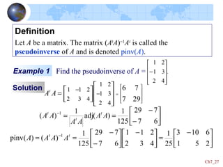
33. Ch7_33
The least squares solution is
Thus a = 1, b = 0.7.
The equation of the least-squares line for this data is
y = 1 + 0.7x






=














−−
−
=−
7.0
1
6226
1001020
20
1
])[(
4
2
4
1
1
ytt
AAA
Figure 7.11

34. Ch7_34
Example 4
Find the least-squares parabola for the following data points.
(1, 7), (2, 2), (3, 1), (4, 3)
Solution
Let the equation of the parabola be y = a + bx + cx2
. Substituting
for these points into the equation of the parabola, we get the
system
3164
193
242
7
=++
=++
=++
=++
cba
cba
cba
cba
We find the least squares solution. The matrix of coefficients A
and column vector y are as follows.








=








=
3
1
2
7
1641
931
421
111
and yA
It can be shown that






==
−−
−−
−−
−
5555
19272331
15251545
1
20
1
)()(pinv tt
AAAA

35. Ch7_35
The least squares solution is
Thus a = 15.25, b = -10.05, c = 1.75.
The equation of the least-squares parabola for these data points is
y = 15.25 – 10.05x + 1.75x2








=














= −
−−
−−
−−
−
75.1
05.10
25.15
3
1
2
7
5555
19272331
15251545
1
20
1
])[( ytt
AAA
Figure 7.12

36. Ch7_36
Let (x1, y1), …, (xn, yn) be a set of n data points. Let y = a0 + … +
amxm be a polynomial of degree m (n > m) that is to be fitted to
these points. Substituting these points into the polynomial leads
to a system Ax = y of n linear equations in the m variables a0, …,
am, where
The least-squares solution to
this system gives the coefficients
of the least-squares polynomial
for these data points.
Theorem 7.1










=










=
n
m
nn
m
y
y
xx
xx
A 


 111
and
1
1
y
Figure 7.13
y’ is the projection of y onto range(A)

37. Ch7_37
Homework
Exercise 7.4
3, 11, 21