Downloaded 1,505 times
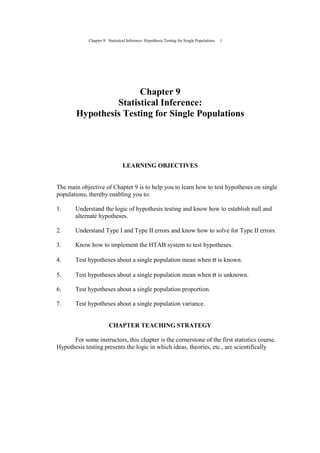


This document provides an outline and overview of Chapter 9 from a statistics textbook. The chapter covers hypothesis testing for single populations, including: - Establishing null and alternative hypotheses - Understanding Type I and Type II errors - Testing hypotheses about single population means when the standard deviation is known or unknown - Testing hypotheses about single population proportions and variances - Solving for Type II errors The chapter teaches students how to implement the HTAB (Hypothesis, Test Statistic, Accept/Reject regions, Boundaries, Conclusion) system to scientifically test hypotheses using statistical techniques like z-tests and t-tests. Key concepts covered include one-tailed and two-tailed tests, critical values, p