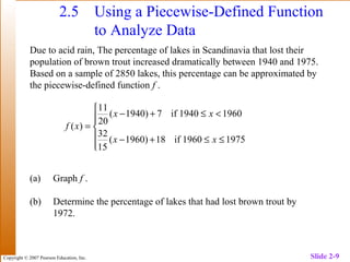
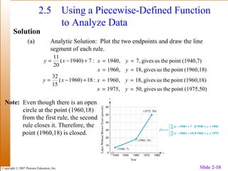
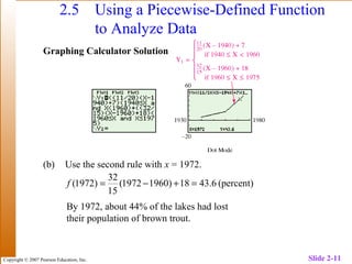
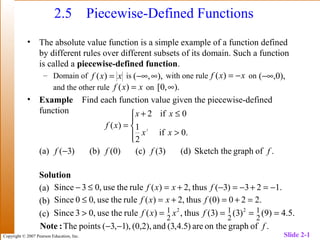
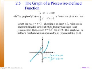
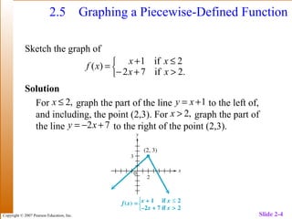
This document discusses piecewise-defined functions and their graphs. It contains the following key points: 1. A piecewise-defined function is a function defined by different rules over different subsets of its domain. An example is given of a piecewise-defined function and evaluating it. 2. The graph of a piecewise-defined function consists of separate pieces joined at the points where the rules change. Examples are given of sketching the graphs. 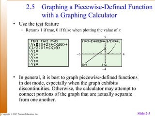3. Graphing calculators can be used to graph piecewise-defined functions by using the test feature to determine which rule applies. 4. Piecewise-defined functions can model real-world scenarios like parking rates that change depending on time.

1. Copyright © 2007 Pearson Education, Inc. Slide 2-1
2.5 Piecewise-Defined Functions
• The absolute value function is a simple example of a function defined
by different rules over different subsets of its domain. Such a function
is called a piecewise-defined function.
– Domain of is with one rule on
and the other rule on
• Example Find each function value given the piecewise-defined
function
Solution
(a)
(b)
(c)
xxf =)( ),,( ∞−∞ xxf −=)( ),0,(−∞
xxf =)( ).,0[ ∞




>
≤+
=
.0if
2
1
0if2
)( 2
xx
xx
xf
.ofgraphSketch the(d))3((c))0((b))3((a) ffff −
.123)3(thus,2)(ruletheuse,03Since −=+−=−+=≤− fxxf
.220)0(thus,2)(ruletheuse,00Since =+=+=≤ fxxf
.5.4)9()3()3(thus,)(ruletheuse,03Since 2
1
2
1
2
1 22
====> fxxf
.ofgraphon theare)5.4,3(and(0,2),),1,3(pointsThe f−−:Note

2. Copyright © 2007 Pearson Education, Inc. Slide 2-2
2.5 The Graph of a Piecewise-Defined
Function
(d) The graph of
Graph the ray choosing x so that with a solid
endpoint (filled in circle) at (0,2). The ray has slope 1 and
y-intercept 2. Then, graph for This graph will be
half of a parabola with an open endpoint (open circle) at (0,0).
time.aatpieceonedrawnis
0if
2
1
0if2
)( 2




>
≤+
=
xx
xx
xf
,2+= xy ,0≤x
2
2
1
xy = .0>x
Figure 51 pg 2-117

3. Copyright © 2007 Pearson Education, Inc. Slide 2-3
2.5 Graphing a Piecewise-Defined Function
with a Graphing Calculator
• Use the test feature
– Returns 1 if true, 0 if false when plotting the value of x
• In general, it is best to graph piecewise-defined functions
in dot mode, especially when the graph exhibits
discontinuities. Otherwise, the calculator may attempt to
connect portions of the graph that are actually separate
from one another.

4. Copyright © 2007 Pearson Education, Inc. Slide 2-4
2.5 Graphing a Piecewise-Defined Function
Sketch the graph of
Solution
For graph the part of the line to the left of,
and including, the point (2,3). For graph the part of
the line to the right of the point (2,3).



>+−
≤+
=
.2if72
2if1
)(
xx
xx
xf
1+= xy
72 +−= xy
,2≤x
,2>x

5. Copyright © 2007 Pearson Education, Inc. Slide 2-5
2.5 The Greatest Integer (Step) Function
Example Evaluate for (a) –5, (b) 2.46, and (c) –6.5
Solution (a)
(b)
(c)
Using the Graphing Calculator
The command “int” is used by many graphing calculators
for the greatest integer function.



=
integerannotisifthanlessintegergreatestthe
integeranisif
xx
xx
5−
2
7−
§ ¨( )f x x=
§ ¨x

6. Copyright © 2007 Pearson Education, Inc. Slide 2-6
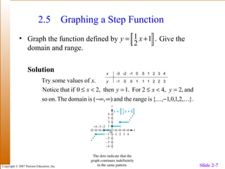
2.5 The Graph of the Greatest Integer
Function
– Domain:
– Range:
• If using a graphing calculator, put the calculator in dot mode.
[ ]||)( xxf =
),( ∞−∞
},3,2,1,0,1,2,3,{}integeranis{  −−−=xx
Figure 58 pg 2-124

7. Copyright © 2007 Pearson Education, Inc. Slide 2-7
2.5 Graphing a Step Function
• Graph the function defined by Give the
domain and range.
Solution
Try some values of x.
.1
2
1



 += xy
x -3 -2 -1 0 .5 1 2 3 4
y -1 0 0 1 1 1 2 2 3
}.,2,1,0,1,{israngetheand),(isdomainTheon.so
and,2,42For.1then,20ifthatNotice
 −∞−∞
=<≤=<≤ yxyx

8. Copyright © 2007 Pearson Education, Inc. Slide 2-8
2.5 Application of a Piecewise-Defined
Function
Downtown Parking charges a $5 base fee for parking through 1 hour, and
$1 for each additional hour or fraction thereof. The maximum fee for 24
hours is $15. Sketch a graph of the function that describes this pricing
scheme.
Solution
Sample of ordered pairs (hours,price): (.25,5), (.75,5), (1,5), (1.5,6), (1.75,6).
During the 1st
hour: price = $5
During the 2nd
hour: price = $6
During the 3rd
hour: price = $7
During the 11th
hour: price = $15
It remains at $15 for the rest of
the 24-hour period.
Plot the graph on the interval (0,24]. Figure 62 pg 2-127


9. Copyright © 2007 Pearson Education, Inc. Slide 2-9
2.5 Using a Piecewise-Defined Function
to Analyze Data
Due to acid rain, The percentage of lakes in Scandinavia that lost their
population of brown trout increased dramatically between 1940 and 1975.
Based on a sample of 2850 lakes, this percentage can be approximated by
the piecewise-defined function f .
(a) Graph f .
(b) Determine the percentage of lakes that had lost brown trout by
1972.






≤≤+−
<≤+−
=
19759601if18)1960(
15
32
19609401if7)1940(
20
11
)(
xx
xx
xf

10. Copyright © 2007 Pearson Education, Inc. Slide 2-10
2.5 Using a Piecewise-Defined Function
to Analyze Data
Solution
(a) Analytic Solution: Plot the two endpoints and draw the line
segment of each rule.
Note: Even though there is an open
circle at the point (1960,18)
from the first rule, the second
rule closes it. Therefore, the
point (1960,18) is closed.
(1960,18)pointtheusgives,18,1960
(1940,7)pointtheusgives,7,1940
==
==
yx
yx:7)1940(
20
11
+−= xy
(1975,50)pointtheusgives,50,1975
(1960,18)pointtheusgives,18,1960
==
==
yx
yx:18)1960(
15
32
+−= xy
Figure 63 pg 2-128

11. Copyright © 2007 Pearson Education, Inc. Slide 2-11
2.5 Using a Piecewise-Defined Function
to Analyze Data
Graphing Calculator Solution
(b) Use the second rule with x = 1972.
(percent)6.4318)19601972(
15
32
)1972( =+−=f
By 1972, about 44% of the lakes had lost
their population of brown trout.