Chapter 6 - Integer Linear Programming : S-1
———————————————————————————————————————————
—
Chapter 6
Integer Linear Programming
1. The optimal solutions to an LP problem occur at extreme points of the feasible region. There are a finite
number of such extreme points for any given problem and they can be located and searched very
efficiently. The optimal solution to an ILP does not necessarily occur at an extreme point of the
relaxed feasible region, making it more difficult to locate these points.
2. M12 = MIN( 200/1, 1520/9, 2650/12) = 168.9
M22 = MIN( 200/1, 1520/6, 2650/16) = 165.7
3. a. X1 + X2 + X4 + X6 = 2
b. X2 - X3 = 0
c. 2X5 - X3 - X4 ≤ 0
d. X2 + X4 - X5 ≤ 1
4. a. See file: Prb6_4.xls
b. Select projects 2, 3 & 5. Total NPV = $573,000.
5. a. It would merely serve to reduce his net profit by $1,000. Since he must incur this cost regardless of
what kind of hot tub he makes there is not reason to include this cost in the formulation of the
model.
b. MAX 350 X1 + 300 X2 - 900 Y1 - 800 Y2
ST 1 X1 + 1 X2 ≤ 200
9 X1 + 6 X2 ≤ 1,520
12 X1 + 16 X2 ≤ 2,650
X1 - M Y1 ≤ 0
X2 - M Y2 ≤ 0
X1, X2 must be nonnegative integers
Y1,Y2 must be binary
6. a. MIN X1 + X2 + X3 + X4 + X5 + X6 + X7
ST X2 + X3 + X4 + X5 + X6 ≥ 18
X3 + X4 + X5 + X6 + X7 ≥ 17
X1 + X4 + X5 + X6 + X7 ≥ 16
X1 + X2 + X5 + X6 + X7 ≥ 16
X1 + X2 + X3 + X6 + X7 ≥ 16
X1 + X2 + X3 + X4 + X7 ≥ 14
X1 + X2 + X3 + X4 + X5 ≥ 19
Xi ≥ 0 & integer
b. See file Prb6_6.xls
c. X1 =5, X2 =2, X3 =6, X4 =2, X5 =6, X6 =2, X7 =1 (alternate optimal solutions exist).
d. 3
7. a. MIN: 32X1 + 80X2 + 32X3 + 80X4 + 32X5 + 80X6 + 32X7
ST X1 + X2 ≥ 11
X1 + X2 ≥ 11
X1 + X2 ≥ 11
X1 + X2 ≥ 11
Chapter 6 - Integer Linear Programming : S-2
———————————————————————————————————————————
—
X2 + X3 + X4 ≥ 24
X2 + X3 + X4 ≥ 24
X2 + X3 + X4 ≥ 16
X2 + X3 + X4 ≥ 16
X4 + X5 + X6 ≥ 10
X4 + X5 + X6 ≥ 10
X4 + X5 + X6 ≥ 22
X4 + X5 + X6 ≥ 22
X6 + X7 ≥ 17
X6 + X7 ≥ 17
X6 + X7 ≥ 6
X6 + X7 ≥ 6
X2 + X4 ≥ 0.3*(X2+X3+X4)
X4 + X6 ≥ 0.3*(X4+X5+X6)
X2 ≥ 1
X6 ≥ 1
Xi ≥ 0 & integer
b. See file Prb6_7.xls
c. X1=9, X2=2, X3=16, X4=6, X5=15, X6=1, X7=16
Total cost = $2,512
8.
Year
1 2 3 4 5
Minimum
Capacity in MW 780 860 950 1060 1180
a. Let Xij = # of generators of size j purchased in year i.
MIN 300 X1,10 + 460 X1,25 + 670 X1,50 + 950 X1,100 +
250 X2,10 + 375 X2,25 + 558 X2,50 + 790 X2,100 +
200 X3,10 + 350 X3,25 + 465 X3,50 + 670 X3,100 +
170 X4,10 + 280 X4,25 + 380 X4,50 + 550 X4,100 +
145 X5,10 + 235 X5,25 + 320 X5,50 + 460 X5,100
ST 750 + 10 X1,10 + 25 X1,25 + 50 X1,50 + 100 X1,100 ≥ 780
750 + 10 (X1,10 + X2,10 ) + 25 (X1,25 + X2,25) + 50 (X1,50 + X2,50 ) + 100 (X1,100 + X2,100) ≥ 860
750 + 10 (X1,10 + X2,10 + X3,10 ) + 25 (X1,25 + X2,25 + X3,25)
+ 50 (X1,50 + X2,50 + X3,50) + 100 (X1,100 + X2,100 + X3,100) ≥ 950
750 + 10 (X1,10 + X2,10 + X3,10 + X4,10) + 25 (X1,25 + X2,25 + X3,25 + X4,25)
+ 50 (X1,50 + X2,50 + X3,50 + X4,50) + 100 (X1,100 + X2,100 + X3,100 + X4,100) ≥ 1060
750 + 10 (X1,10 + X2,10 + X3,10 + X4,10 + X5,10) + 25 (X1,25 + X2,25 + X3,25 + X4,25 + X5,25)
+ 50(X1,50 + X2,50 + X3,50+ X4,50 + X5,50)+100(X1,100 + X2,100 + X3,100 + X4,100 + X5,100)≥1060
Xij ≥ 0 and integer
b. See file: Prb6_8.xls
c. X1,100 = X2,10 = X3,100 = X4,100 = X5,25 = X5,100 = 1, Total Cost = $3,115,000
9. a. MIN 450 X1 + 650 X2 + 550 X3 + 500 X4 + 525 X5
ST X1 + X3 ≥ 1
X1 + X2 + X4 + X5 ≥ 1
X2 + X4 ≥ 1
Chapter 6 - Integer Linear Programming : S-3
———————————————————————————————————————————
—
X3 + X5 ≥ 1
X1 + X2 ≥ 1
X3 + X5 ≥ 1
X4 + X5 ≥ 1
All Xi are binary
where:
X1 = 1 if Sanford is selected, 0 otherwise
X2 = 1 if Altamonte is selected, 0 otherwise
X3 = 1 if Apopka is selected, 0 otherwise
X4 = 1 if Casselberry is selected, 0 otherwise
X5 = 1 if Maitland is selected, 0 otherwise
b. See file: Prb6_9.xls
c. X1= X4X5 =1 (Build at Sanford and Casselberry & Maitland)
Minimum total cost = $1,475,000
10. a. X1 = batches of CD players to produce
X2 = batches of tape decks to produce
X3 = batches of stereo tuners to produce
MAX (75*150) X1 + (50*150) X2 + (40*150) X3
ST (3*150) X1 + (2*150) X2 + (1*150) X3 ≤ 400,000
50,000/150 ≤ X1 ≤ 150,000/150
50,000/150 ≤ X2 ≤ 100,000/150
50,000/150 ≤ X3 ≤ 90,000/150
b. See file: Prb6_10.xls
c. X1=334, X2=532, X3=600
Maximum profit = $11,347,500
11. a. MIN 21X1 + 23X2 + 25X3 + 24X4 + 20X5 + 26X6
+ 1000Y1 + 950Y2 + 875Y3 + 850Y4 + 800Y5 + 700Y6
ST X1 + X2 + X3 + X4 + X5 + X6 = 1800
X1 - 500 Y1 ≤ 0
X2 - 600 Y2 ≤ 0
X3 - 750 Y3 ≤ 0
X4 - 400 Y4 ≤ 0
X5 - 600 Y5 ≤ 0
X6 - 800 Y6 ≤ 0
Xi ≥ 0
All Yi are binary
b. See file: Prb6_11.xls
c. X1=500, X2=600, X4=100, X5=600
Total cost = $42,300
12. a. Xij = 1 if item i is sold in year j, 0 otherwise
Chapter 6 - Integer Linear Programming : S-4
———————————————————————————————————————————
—
MAX ΣΣCijXij
S.T. ΣXij = 1, for each item i
ΣCijXij ≥ 30, for each year j
b. See file: Prb6_12.xls
c. Total Cash Received $275,000
Year Item Sold
1 Car
2 Golf Clubs
3 Portrait
4 Desk
5 Piano
5 Humidor
13. a. Let Xi = 1 if project i is selected, 0 otherwise
MAX 650 X1 + 550 X2 + 600 X3 + 450 X4 + 375 X5 + 525 X6 + 750 X7
ST 7 X1 + 6 X2 + 9 X3 + 5 X4 + 6 X5 + 4 X6 + 8 X7 ≤ 20
250 X1 + 175 X2 + 300 X3 + 150 X4 + 145 X5 + 160 X6 + 325 X7 ≤ 950
X2 + X6≤ 1 (implemented as X2 ≤ 1-X6 )
b. See file: Prb6_13.xls
c. X1=X6=X7=1, Total NPV = $1,925,000
14. a. Let Xij = bushels (in 1000s) shipped from grove i to processing plant j
Yij = 1 if Xij ≥ 0, 0 otherwise
MIN $168 Y14 + $400 Y15 + $320 Y16
$280 Y24 + $240 Y25 + $176 Y26
$440 Y34 + $160 Y35 + $200 Y36
ST X14 + X15 + X16 = 275
X24 + X25 + X26 = 400
X34 + X35 + X36 = 300
X14 + X24 + X34 ≤ 200
X15 + X25 + X35 ≤ 600
X16 + X26 + X36 ≤ 225
Xij - MijYij ≤ 0
Xij ≥ 0
Yij binary
Note: Mij = MIN(supply of i, capacity of j)
b. See file: Prb6_14.xls
c. The solution is: X15= 275, X24= 200, X26= 200, X35= 300,
Y15= 1, Y24= 1, Y26= 1, Y35= 1.
Minimum trucking cost = $1,016.
Chapter 6 - Integer Linear Programming : S-5
———————————————————————————————————————————
—
15. a. X0 = number of efficiency apartments to build
X1 = number of 1-bedroom apartments to build
X2 = number of 2-bedroom apartments to build
X3 = number of 3-bedroom apartments to build
MAX 350 X0 + 450 X1 + 550 X2 + 750 X3
ST X0 + X1 + X2 + X3 ≤ 40
500X0 + 700X1 + 800X2 + 1,000X3 ≤ 40,000
0 ≤ X0 ≤ 40
5 ≤ X1 ≤ 15
8 ≤ X2 ≤ 22
0 ≤ X3 ≤ 10
Xi integer
b. See file: Prb6_15.xls
c. X0 = 0 , X1= 8 , X2 = 22 , X3 = 10
Maximum monthly rental income = $23,200
d. There are three binding constraints: the constraint restricting the total number of units to 40, the
upper limit of 22 on the number of 2-bedroom apartments, and the upper limit of 10 on the number
of 3-bedroom apartments.
16. a. The possible cutting patterns are summarized below:
Cutting Number of boards cut
Pattern 7 ft 9 ft 11 ft
1 3 0 0
2 2 1 0
3 2 0 1
4 1 2 0
5 0 1 1
6 0 0 2
Xi = number of boards to which cutting pattern i is applied
MIN X1 + X2 + X3 + X4 + X5 + X6
ST 3X1 + 2X2 + 2X3 + 1X4 + 0X5 + 0X6 ≥ 5,000
0X1 + 1X2 + 0X3 + 2X4 + 1X5 + 0X6 ≥ 1,200
0X1 + 0X2 + 1X3 + 0X4 + 1X5 + 2X6 ≥ 300
Xi ≥ 0 & integer
b. See file: Prb6_16.xls
c. X1 = 1267, X3 = 300, X4 = 600, Total boards cut = 2167 (other solutions exist)
17. a. The possible cutting patterns are summarized below:
Cutting Pattern Roll Size 4 ft Strips 9 ft Strips 12 ft Strips
1 14 ft 3 0 0
2 14 ft 1 1 0
3 14 ft 0 0 1
Chapter 6 - Integer Linear Programming : S-6
———————————————————————————————————————————
—
4 18 ft 4 0 0
5 18 ft 2 1 0
6 18 ft 1 0 1
7 18 ft 0 2 0
Xi = number of rolls to which cutting pattern i is applied
MIN 1,000(X1 + X2 + X3 ) + 1,400( X4 + X5 + X6 + X7)
ST 100(3X1 + 1X2 + 0X3 + 4X4 + 2X5 + 1X6 + 0X7) ≥ 4,000
100(0X1 + 1X2 + 0X3 + 0X4 + 1X5 + 0X6 + 2X7) ≥ 20,000
100(0X1 + 0X2 + 1X3 + 0X4 + 0X5 + 1X6 + 0X7) ≥ 9,000
Xi ≥ 0
b. See file: Prb6_17.xls
c. X2 = 40, X3 = 90, X7 = 80
Minimum cost = $242,000
18. a. Let Pij = production at plant i allocated to meet demand for customer j
Yi= 1 if any Xij ≥ 0, 0 otherwise
MIN 35 P1X + 30 P1Y + 45 P1Z + 45 P2X + 40 P2Y + 50 P2Z + 70 P3X + 65 P3Y
+ 50 P3Z + 20 P4X + 45 P4Y + 25 P4Z + 65 P5X + 45 P5Y + 45 P5Z
+ 1000 (1,325 Y1 + 1,100 Y2 + 1,500 Y3 + 1,200 Y4 + 1,400 Y5)
ST P1X + P1Y + P1Z ≤ 40,000 Y1
P2X + P2Y + P2Z ≤ 30,000 Y2
P3X + P3Y + P3Z ≤ 50,000 Y3
P4X + P4Y + P4Z ≤ 20,000 Y4
P5X + P5Y + P5Z ≤ 40,000 Y5
P1X + P2X + P3X + P4X + P5X ≥ 40,000
P1Y + P2Y + P3Y + P4Y + P5Y ≥ 25,000
P1Z + P2Z + P3Z + P4Z + P5Z ≥ 35,000
Pij ≥ 0
Yi binary
b. See file: Prb6_18.xls
c The solution is: Build plants at locations 1, 4 and 5 (i.e., Y1=Y4=Y5 = 1).
P1X=P1Y=P4X=20,000, P5Y=5,000, P5Z=35,000.
Total cost = $7,425,000.
19. a. Additional Constraints: Y1+Y2 ≤ 1 and Y4+Y5 ≤ 1 (implement as Y1≤ 1-Y2 and Y4≤ 1-Y5)
b. See file: Prb6_19.xls
c. The solution is: Build plants at locations 1, 3 and 4 (i.e., Y1=Y3=Y4 = 1).
P1X=15,000, P1Y=25,000, P3X=5,000, P3Z=35,000, P4X=20,000.
Total cost = $7,800,000.
20. a. MIN 13 A1+ 9 B1+ 10 C1+ 11 A1+ 12 B2+ 8 C2 +
55 YA1+ 93 YB1+ 60 YC1+ 65 YA2+ 58 YB2+ 75 YC2
ST A1+ A2 = 3
Chapter 6 - Integer Linear Programming : S-7
———————————————————————————————————————————
—
B1+ B2 = 7
C1+ C2 = 4
0.4 A1+ 1.1 B1+ 0.9 C1≤ 8
0.5 A2+ 1.2 B2+ 1.3 C2≤ 6
A1- 3YA1 ≤ 0
B1- 7YB1 ≤ 0
C1- 4YC1 ≤ 0
A2- 3YA2 ≤ 0
B2- 7YB2 ≤ 0
C2- 4YC2 ≤ 0
Ai, Bi, Ci ≥ and integer
Yij binary
b. See file: Prb6_20.xls
c. The optimal solution is: A2=3, B1=4, B2=3,C1=4, YA2=YB1=YB2=YC1=1
Total cost = $421
21. a. Let X1j = barrels of crude to buy from TX allocated to the production of product j
X2j = barrels of crude to buy from OK allocated to the production of product j
X3j = barrels of crude to buy from PA allocated to the production of product j
X4j = barrels of crude to buy from AL allocated to the production of product j
Yi = 1 if Xi > 0 and 0 otherwise
MIN 22 X1 + 21 X2 + 22 X3 + 23 X4 + 1500 Y1 + 1700 Y2 + 1500 Y3 + 1400 Y4
ST 2.00 X11 + 1.80 X21 + 2.30 X31 + 2.10 X41 ≥ 750
2.80 X12 + 2.30 X22 + 2.20 X32 + 2.60 X42 ≥ 800
1.70 X13 + 1.75 X23 + 1.60 X33 + 1.90 X43 ≥ 1000
2.40 X14 + 1.90 X24 + 2.60 X34 + 2.40 X44 ≥ 300
X1 = X11 + X12 + X13 + X14
X2 = X21 + X22 + X23 + X24
X3 = X31 + X32 + X33 + X34
X4 = X41 + X42 + X43 + X44
X1 - 1500 Y1 ≤ 0
X2 - 2000 Y2 ≤ 0
X3 - 1500 Y3 ≤ 0
X4 - 1800 Y4 ≤ 0
X1 - 500 Y1 ≥ 0
X2 - 500 Y2 ≥ 0
X3 - 500 Y3 ≥ 0
X4 - 500 Y4 ≥ 0
b. See file: Prb6_21.xls
c. Purchase 2,000 barrels from Oklahoma and 850 barrels from Pennsylvania.
Total cost = $63,900.
22. a. MIN S1 + S2 + S3
S.T. X11 + X12 + X13 + X14 + X15 + S1 = 2700
Chapter 6 - Integer Linear Programming : S-8
———————————————————————————————————————————
—
X21 + X22 + X23 + X24 + X25 + S2 = 3500
X31 + X32 + X33 + X34 + X35 + S3 = 4200
Y11 + Y21 + Y31 ≤ 1
Y12 + Y22 + Y32 ≤ 1
Y13 + Y23 + Y33 ≤ 1
Y14 + Y24 + Y34 ≤ 1
Y15 + Y25 + Y35 ≤ 1
Xi1 - 2500Yi1 ≤ 0, i=1 to 3
Xi2 - 2000Yi2 ≤ 0, i=1 to 3
Xi3 - 1500Yi3 ≤ 0, i=1 to 3
Xi4 - 1800Yi4 ≤ 0, i=1 to 3
Xi5 - 2300Yi5 ≤ 0, i=1 to 3
Yj binary
Xi ≥ 0
b. See file: Prb6_22.xls
c. Compartment 1, 2500 gallons of diesel
Compartment 2, 2000 gallons of regular unleaded
Compartment 3, 1500 gallons of regular unleaded
Compartment 4, 1800 gallons of premium unleaded
Compartment 5, 2300 gallons of premium unleaded
Minimum shortage = 300 gallons
23. a. A = Amount to invest in investment A
B = Amount to invest in investment B
C = Amount to invest in investment C
D = Amount to invest in investment D
E = Amount to invest in investment E
M1 = Amount to invest in the money market in 2001
M2 = Amount to invest in the money market in 2002
M3 = Amount to invest in the money market in 2003
MAX 1.3 B + 1.65 C + 1.3 D + 1.05 M3
ST A + C + E + M1 = 1,000,000
0.45 A + 1.05 M1 - B – M2 = 0
1.05 A + 1.25 E + 1.05 M2 – D – M3 = 0
A - M YA ≤ 0
B - M YB ≤ 0
C - M YC ≤ 0
D - M YD ≤ 0
E - M YE ≤ 0
A - 50000 YA ≥ 0
B - 50000 YB ≥ 0
C - 50000 YC ≥ 0
D - 50000 YD ≥ 0
E - 50000 YE ≥ 0
A, B, C, D, E, M1, M2, M3 ≥ 0
Yi binary
b. See file: Prb6_23.xls
c. A=100,000, B= 0, C=0, D=152,250, E=0, M1=0, M2=45,000, M3=0
Maximum amount of money at the beginning of 2004 = $197,925
Chapter 6 - Integer Linear Programming : S-9
———————————————————————————————————————————
—
24. a. Let Bi = beginning inventory in week i
Ni = the number of batches ordered in week i
Ei = inventory held at the end of week i
Di = demand in week i
Yi = 1 if Bi > 0, 0 otherwise
MIN 125*(N1+ N2+ N3+ N4) + 50*(Y1+ Y2+ Y3+ Y4) + 15*(E1+ E2+ E3+ E4)/100
ST Bi=Ei-1, i=2,3,4
Ei = Bi + 100*Ni - Di , i=1,2,3,4
Ni - M Yi≤ 0
Ei ≥ 0
Yi binary
Ni ≥ 0 and integer
b. See file: Prb6_24.xls
c. The optimal solution is: N1=6, N3=5, Y1=1, Y3=1.
Minimum total cost = $1,565.
25. a. Let Xi = 1 if design change i is selected, 0 otherwise
MIN 150 X1 + 350 X2 + 50 X3 + 450 X4 + 90 X5 + 35 X6 + 650 X7 + 75 X8 + 110 X9 + 30 X10
ST 50X1 + 75 X2 + 25 X3 + 150 X4 + 60 X5 + 95 X6 + 200 X7 + 40 X8 + 80 X9 + 30 X10 ≥ 400
X4 ≤ 1 - X7
Xi binary
b. See file: Prb6_25.xls
c. The optimal solution is: X4 = X5 = X6 = X9 = X10 = 1.
Minimum total cost = $715,000.
26. a. See file Prb6_26.xls
b. Build Red Snappers at sites 4, 8 & 9. Build Olive Groves at sites 1, 6 & 10. NPV=$105.8.
c. See file Prb6_26.xls
d. Build Red Snappers at sites 4, 7 & 9. Build Olive Groves at sites 1, 6 & 10. NPV=$100.3.
27. a. MAX 70(X11+X21+X31)+50(X12+X22+X32)+60(X13+X23+X33)+80(X14+X24+X34)
ST X11+X21+X31 ≤ 4800
X12+X22+X32 ≤ 2500
X13+X23+X33 ≤ 1200
X14+X24+X34 ≤ 1700
X11+X12+X13+X14 ≤ 3000
X21+X22+X23+X24 ≤ 6000
X31+X32+X33+X34 ≤ 4000
40X11+25X12+60X13+55X14 ≤ 145000
40X21+25X22+60X23+55X24 ≤ 180000
40X31+25X32+60X33+55X34 ≤ 155000
0.9(X31+X32+X33+X34) ≤ X11+X12+X13+X14 ≤ 1.1(X31+X32+X33+X34)
0.4ΣΣXij ≤ X21+X22+X23+X24 ≤ 0.6ΣΣXij
Xij ≤ MjYij, ∀ ij
ΣYij ≤ 1, ∀ i
Chapter 6 - Integer Linear Programming : S-10
———————————————————————————————————————————
—
Xij ≥ 0
Yij binary
b. See file Prb6_27.xls
c. Load 4500 tons of commodity 1 in center hold (X21=4500), 1888.89 tons of commodity 2 in rear
hold (X32=1888.89), 1700 tons of commodity 4 in forward hold (X14=1700). Profit = $545,444.
28. a. See file: Prb6_28.xls
b. Build towers in areas 8, 11, 19 & 22; Profit = $377 thousand.
c. Build towers in areas 3, 5, 6, 14, 17, 22, 25; Profit = $219 thousand.
29. a. Let Xi = 1 if an ambulance is located in region i
MAX 205 X1 + 190 X2 + 136 X3 + 162 X4 + 116 X5
ST 1 X1 + 1 X2 + 0 X3 + 1 X4 + 1 X5 ≥ 1
1 X1 + 1 X2 + 1 X3 + 1 X4 + 0 X5 ≥ 1
0 X1 + 1 X2 + 1 X3 + 0 X4 + 1 X5 ≥ 1
1 X1 + 1 X2 + 0 X3 + 1 X4 + 0 X5 ≥ 1
1 X1 + 0 X2 + 1 X3 + 0 X4 + 1 X5 ≥ 1
1 X1 + 1 X2 + 1 X3 + 1 X4 + 1 X5 ≤ 2
Xi binary
b. See file: Prb6_29.xls
c. The optimal solution is: X1 = X2 = 1.
A total of 395,000 people can be reached within 4 minutes using these locations.
Chapter 6 - Integer Linear Programming : S-11
———————————————————————————————————————————
—
30. a. See file Prb6_30.xls
b.
State Week
AZ 6
CA 6
CT 2
GA 3
IL 5
MA 4
ME 6
MN 4
MT 5
NC 1
NJ 4
NV 1
OH 2
OR 4
TX 3
VA 1
Maximum pieces processed in any week: 353,856
31. a. See file Prb6_31.xls
b. Operate plants 2, 3, 5 & 6, warehouses 3 & 4. Total cost = $855,000
c. See file Prb6_31.xls
32. Errata: Assume the van can carry a maximum of 800 units of blood (rather than 200).
a. See file: Prb6_32.xls
b.
Chapter 6 - Integer Linear Programming : S-12
———————————————————————————————————————————
—
c.
33. a. See file Prb6_33.xls. Place hubs in Andersen, Berekley, Dillon, Edgefield, Hampton,. Kershaw,
Orangeburg & Union. Total hubs = 8, Total coverage = 55.
b. See file Prb6_29.xls. Place hubs in Bamberg, Colleton, Florence, Greenville, Greenwood,
Hampton, Kershaw, Marion, Orangeburg & Union. Total hubs = 10, Total coverage = 77.
34.
X = 2.25
1
X = 1.50
2
Obj = 25.5
X = 2.0
1
X = 1.67
2
Obj = 25.3
X = 3.0
1
X = 0.0
2
Obj = 18
X <= 2
1 X >= 3
1
X = 2.0
1
X = 1.0
2
Obj = 20
X = 1.5
1
X = 2.0
2
Obj = 25.0
X <= 1
2
X >= 2
2
X = 1.0
1
X = 2.33
2
Obj = 24.6
X = 1.0
1
X = 2.0
2
Obj = 22.0
X = 0.0
1
X = 3.0
2
Obj = 24.0
Infeasible
X <= 1
1 X >= 2
1
X >= 3
2
X <= 2
2
optimal solution
Errata: In the first printing of SMDA 5ed the problem on page 291 is labeled 34 when it should be 35.
Chapter 6 - Integer Linear Programming : S-13
———————————————————————————————————————————
—
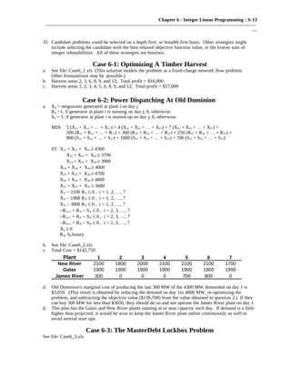
35. Candidate problems could be selected on a depth first, or breadth first basis. Other strategies might
include selecting the candidate with the best relaxed objective function value, or the lowest sum of
integer infeasibilities. All of these strategies are heuristic.
Case 6-1: Optimizing A Timber Harvest
a. See file: Case6_1.xls (This solution models the problem as a fixed-charge network flow problem.
Other formulations may be possible.)
b. Harvest areas 2, 3, 6, 8, 9, and 12; Total profit = $16,000
c. Harvest areas 1, 2, 3, 4, 5, 6, 8, 9, and 12; Total profit = $17,000
Case 6-2: Power Dispatching At Old Dominion
a. Xij = megawatts generated at plant i on day j
Rij =1, if generator at plant i is running on day j; 0, otherwise.
Sij = 1, if generator at plant i is started-up on day j; 0, otherwise.
MIN 5 (X11 + X12 + … + X17) + 4 (X21 + X22 + … + X27) + 7 (X31 + X32 + … + X37) +
200 (R11 + R12 + … + R17) + 300 (R21 + R22 + … + R27) + 250 (R31 + R32 + … + R37) +
800 (S11 + S12 + … + S17) + 1000 (S21 + S22 + … + S27) + 700 (S31 + S32 + … + S37)
ST X11 + X21 + X31 ≥ 4300
X12 + X22 + X32 ≥ 3700
X13 + X23 + X33 ≥ 3900
X14 + X24 + X34 ≥ 4000
X15 + X25 + X35 ≥ 4700
X16 + X26 + X36 ≥ 4800
X17 + X27 + X37 ≥ 3600
X1i − 2100 R1i ≤ 0 , i = 1, 2, …, 7
X2i − 1900 R2i ≤ 0 , i = 1, 2, …, 7
X3i − 3000 R3i ≤ 0 , i = 1, 2, …, 7
−R1,i-1 + R1i − S1i ≤ 0 , i = 2, 3, …, 7
−R2,i-1 + R2i − S2i ≤ 0 , i = 2, 3, …, 7
−R3,i-1 + R3i − S3i ≤ 0 , i = 2, 3, …, 7
Xij ≥ 0
Rij, Sij binary
b. See file: Case6_2.xls
c. Total Cost = $142,750
Plant 1 2 3 4 5 6 7
New River 2100 1800 2000 2100 2100 2100 1700
Galax 1900 1900 1900 1900 1900 1900 1900
James River 300 0 0 0 700 800 0
d. Old Dominion's marginal cost of producing the last 300 MW of the 4300 MW demanded on day 1 is
$3,050. (This result is obtained by reducing the demand on day 1to 4000 MW, re-optimizing the
problem, and subtracting the objective value ($139,700) from the value obtained in question 2.) If they
can buy 300 MW for less than $3050, they should do so and not operate the James River plant on day 1.
d. This plan has the Galax and New River plants running at or near capacity each day. If demand is a little
higher than projected, it would be wise to keep the James River plant online continuously as well to
avoid several start ups.
Case 6-3: The MasterDebt Lockbox Problem
See file: Case6_3.xls
Chapter 6 - Integer Linear Programming : S-14
———————————————————————————————————————————
—
a. Use Dallas and New York, Total cost = $224,000
b. Use Sacramento and Atlanta, Total cost = $225,750
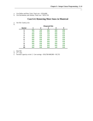
Case 6-4: Removing More Snow in Montreal
a. See file: Case6_4.xls
b.
Disposal Site
Sector 1 2 3 4 5
1 0.0 1.0 0.0 0.0 0.0
2 1.0 0.0 0.0 0.0 0.0
3 0.0 0.0 1.0 0.0 0.0
4 0.0 0.0 1.0 0.0 0.0
5 0.0 0.0 1.0 0.0 0.0
6 0.0 0.0 0.0 1.0 0.0
7 0.0 0.0 0.0 1.0 0.0
8 0.0 0.0 0.0 0.0 1.0
9 1.0 0.0 0.0 0.0 0.0
10 0.0 0.0 0.0 1.0 0.0
c. $54,700
d. 250
= lots
e. Increase capacity at site 2. Cost savings = $54,700-$48,968 = $5,732

Ch 06

  • 1.
    Chapter 6 -Integer Linear Programming : S-1 ——————————————————————————————————————————— — Chapter 6 Integer Linear Programming 1. The optimal solutions to an LP problem occur at extreme points of the feasible region. There are a finite number of such extreme points for any given problem and they can be located and searched very efficiently. The optimal solution to an ILP does not necessarily occur at an extreme point of the relaxed feasible region, making it more difficult to locate these points. 2. M12 = MIN( 200/1, 1520/9, 2650/12) = 168.9 M22 = MIN( 200/1, 1520/6, 2650/16) = 165.7 3. a. X1 + X2 + X4 + X6 = 2 b. X2 - X3 = 0 c. 2X5 - X3 - X4 ≤ 0 d. X2 + X4 - X5 ≤ 1 4. a. See file: Prb6_4.xls b. Select projects 2, 3 & 5. Total NPV = $573,000. 5. a. It would merely serve to reduce his net profit by $1,000. Since he must incur this cost regardless of what kind of hot tub he makes there is not reason to include this cost in the formulation of the model. b. MAX 350 X1 + 300 X2 - 900 Y1 - 800 Y2 ST 1 X1 + 1 X2 ≤ 200 9 X1 + 6 X2 ≤ 1,520 12 X1 + 16 X2 ≤ 2,650 X1 - M Y1 ≤ 0 X2 - M Y2 ≤ 0 X1, X2 must be nonnegative integers Y1,Y2 must be binary 6. a. MIN X1 + X2 + X3 + X4 + X5 + X6 + X7 ST X2 + X3 + X4 + X5 + X6 ≥ 18 X3 + X4 + X5 + X6 + X7 ≥ 17 X1 + X4 + X5 + X6 + X7 ≥ 16 X1 + X2 + X5 + X6 + X7 ≥ 16 X1 + X2 + X3 + X6 + X7 ≥ 16 X1 + X2 + X3 + X4 + X7 ≥ 14 X1 + X2 + X3 + X4 + X5 ≥ 19 Xi ≥ 0 & integer b. See file Prb6_6.xls c. X1 =5, X2 =2, X3 =6, X4 =2, X5 =6, X6 =2, X7 =1 (alternate optimal solutions exist). d. 3 7. a. MIN: 32X1 + 80X2 + 32X3 + 80X4 + 32X5 + 80X6 + 32X7 ST X1 + X2 ≥ 11 X1 + X2 ≥ 11 X1 + X2 ≥ 11 X1 + X2 ≥ 11
  • 2.
    Chapter 6 -Integer Linear Programming : S-2 ——————————————————————————————————————————— — X2 + X3 + X4 ≥ 24 X2 + X3 + X4 ≥ 24 X2 + X3 + X4 ≥ 16 X2 + X3 + X4 ≥ 16 X4 + X5 + X6 ≥ 10 X4 + X5 + X6 ≥ 10 X4 + X5 + X6 ≥ 22 X4 + X5 + X6 ≥ 22 X6 + X7 ≥ 17 X6 + X7 ≥ 17 X6 + X7 ≥ 6 X6 + X7 ≥ 6 X2 + X4 ≥ 0.3*(X2+X3+X4) X4 + X6 ≥ 0.3*(X4+X5+X6) X2 ≥ 1 X6 ≥ 1 Xi ≥ 0 & integer b. See file Prb6_7.xls c. X1=9, X2=2, X3=16, X4=6, X5=15, X6=1, X7=16 Total cost = $2,512 8. Year 1 2 3 4 5 Minimum Capacity in MW 780 860 950 1060 1180 a. Let Xij = # of generators of size j purchased in year i. MIN 300 X1,10 + 460 X1,25 + 670 X1,50 + 950 X1,100 + 250 X2,10 + 375 X2,25 + 558 X2,50 + 790 X2,100 + 200 X3,10 + 350 X3,25 + 465 X3,50 + 670 X3,100 + 170 X4,10 + 280 X4,25 + 380 X4,50 + 550 X4,100 + 145 X5,10 + 235 X5,25 + 320 X5,50 + 460 X5,100 ST 750 + 10 X1,10 + 25 X1,25 + 50 X1,50 + 100 X1,100 ≥ 780 750 + 10 (X1,10 + X2,10 ) + 25 (X1,25 + X2,25) + 50 (X1,50 + X2,50 ) + 100 (X1,100 + X2,100) ≥ 860 750 + 10 (X1,10 + X2,10 + X3,10 ) + 25 (X1,25 + X2,25 + X3,25) + 50 (X1,50 + X2,50 + X3,50) + 100 (X1,100 + X2,100 + X3,100) ≥ 950 750 + 10 (X1,10 + X2,10 + X3,10 + X4,10) + 25 (X1,25 + X2,25 + X3,25 + X4,25) + 50 (X1,50 + X2,50 + X3,50 + X4,50) + 100 (X1,100 + X2,100 + X3,100 + X4,100) ≥ 1060 750 + 10 (X1,10 + X2,10 + X3,10 + X4,10 + X5,10) + 25 (X1,25 + X2,25 + X3,25 + X4,25 + X5,25) + 50(X1,50 + X2,50 + X3,50+ X4,50 + X5,50)+100(X1,100 + X2,100 + X3,100 + X4,100 + X5,100)≥1060 Xij ≥ 0 and integer b. See file: Prb6_8.xls c. X1,100 = X2,10 = X3,100 = X4,100 = X5,25 = X5,100 = 1, Total Cost = $3,115,000 9. a. MIN 450 X1 + 650 X2 + 550 X3 + 500 X4 + 525 X5 ST X1 + X3 ≥ 1 X1 + X2 + X4 + X5 ≥ 1 X2 + X4 ≥ 1
  • 3.
    Chapter 6 -Integer Linear Programming : S-3 ——————————————————————————————————————————— — X3 + X5 ≥ 1 X1 + X2 ≥ 1 X3 + X5 ≥ 1 X4 + X5 ≥ 1 All Xi are binary where: X1 = 1 if Sanford is selected, 0 otherwise X2 = 1 if Altamonte is selected, 0 otherwise X3 = 1 if Apopka is selected, 0 otherwise X4 = 1 if Casselberry is selected, 0 otherwise X5 = 1 if Maitland is selected, 0 otherwise b. See file: Prb6_9.xls c. X1= X4X5 =1 (Build at Sanford and Casselberry & Maitland) Minimum total cost = $1,475,000 10. a. X1 = batches of CD players to produce X2 = batches of tape decks to produce X3 = batches of stereo tuners to produce MAX (75*150) X1 + (50*150) X2 + (40*150) X3 ST (3*150) X1 + (2*150) X2 + (1*150) X3 ≤ 400,000 50,000/150 ≤ X1 ≤ 150,000/150 50,000/150 ≤ X2 ≤ 100,000/150 50,000/150 ≤ X3 ≤ 90,000/150 b. See file: Prb6_10.xls c. X1=334, X2=532, X3=600 Maximum profit = $11,347,500 11. a. MIN 21X1 + 23X2 + 25X3 + 24X4 + 20X5 + 26X6 + 1000Y1 + 950Y2 + 875Y3 + 850Y4 + 800Y5 + 700Y6 ST X1 + X2 + X3 + X4 + X5 + X6 = 1800 X1 - 500 Y1 ≤ 0 X2 - 600 Y2 ≤ 0 X3 - 750 Y3 ≤ 0 X4 - 400 Y4 ≤ 0 X5 - 600 Y5 ≤ 0 X6 - 800 Y6 ≤ 0 Xi ≥ 0 All Yi are binary b. See file: Prb6_11.xls c. X1=500, X2=600, X4=100, X5=600 Total cost = $42,300 12. a. Xij = 1 if item i is sold in year j, 0 otherwise
  • 4.
    Chapter 6 -Integer Linear Programming : S-4 ——————————————————————————————————————————— — MAX ΣΣCijXij S.T. ΣXij = 1, for each item i ΣCijXij ≥ 30, for each year j b. See file: Prb6_12.xls c. Total Cash Received $275,000 Year Item Sold 1 Car 2 Golf Clubs 3 Portrait 4 Desk 5 Piano 5 Humidor 13. a. Let Xi = 1 if project i is selected, 0 otherwise MAX 650 X1 + 550 X2 + 600 X3 + 450 X4 + 375 X5 + 525 X6 + 750 X7 ST 7 X1 + 6 X2 + 9 X3 + 5 X4 + 6 X5 + 4 X6 + 8 X7 ≤ 20 250 X1 + 175 X2 + 300 X3 + 150 X4 + 145 X5 + 160 X6 + 325 X7 ≤ 950 X2 + X6≤ 1 (implemented as X2 ≤ 1-X6 ) b. See file: Prb6_13.xls c. X1=X6=X7=1, Total NPV = $1,925,000 14. a. Let Xij = bushels (in 1000s) shipped from grove i to processing plant j Yij = 1 if Xij ≥ 0, 0 otherwise MIN $168 Y14 + $400 Y15 + $320 Y16 $280 Y24 + $240 Y25 + $176 Y26 $440 Y34 + $160 Y35 + $200 Y36 ST X14 + X15 + X16 = 275 X24 + X25 + X26 = 400 X34 + X35 + X36 = 300 X14 + X24 + X34 ≤ 200 X15 + X25 + X35 ≤ 600 X16 + X26 + X36 ≤ 225 Xij - MijYij ≤ 0 Xij ≥ 0 Yij binary Note: Mij = MIN(supply of i, capacity of j) b. See file: Prb6_14.xls c. The solution is: X15= 275, X24= 200, X26= 200, X35= 300, Y15= 1, Y24= 1, Y26= 1, Y35= 1. Minimum trucking cost = $1,016.
  • 5.
    Chapter 6 -Integer Linear Programming : S-5 ——————————————————————————————————————————— — 15. a. X0 = number of efficiency apartments to build X1 = number of 1-bedroom apartments to build X2 = number of 2-bedroom apartments to build X3 = number of 3-bedroom apartments to build MAX 350 X0 + 450 X1 + 550 X2 + 750 X3 ST X0 + X1 + X2 + X3 ≤ 40 500X0 + 700X1 + 800X2 + 1,000X3 ≤ 40,000 0 ≤ X0 ≤ 40 5 ≤ X1 ≤ 15 8 ≤ X2 ≤ 22 0 ≤ X3 ≤ 10 Xi integer b. See file: Prb6_15.xls c. X0 = 0 , X1= 8 , X2 = 22 , X3 = 10 Maximum monthly rental income = $23,200 d. There are three binding constraints: the constraint restricting the total number of units to 40, the upper limit of 22 on the number of 2-bedroom apartments, and the upper limit of 10 on the number of 3-bedroom apartments. 16. a. The possible cutting patterns are summarized below: Cutting Number of boards cut Pattern 7 ft 9 ft 11 ft 1 3 0 0 2 2 1 0 3 2 0 1 4 1 2 0 5 0 1 1 6 0 0 2 Xi = number of boards to which cutting pattern i is applied MIN X1 + X2 + X3 + X4 + X5 + X6 ST 3X1 + 2X2 + 2X3 + 1X4 + 0X5 + 0X6 ≥ 5,000 0X1 + 1X2 + 0X3 + 2X4 + 1X5 + 0X6 ≥ 1,200 0X1 + 0X2 + 1X3 + 0X4 + 1X5 + 2X6 ≥ 300 Xi ≥ 0 & integer b. See file: Prb6_16.xls c. X1 = 1267, X3 = 300, X4 = 600, Total boards cut = 2167 (other solutions exist) 17. a. The possible cutting patterns are summarized below: Cutting Pattern Roll Size 4 ft Strips 9 ft Strips 12 ft Strips 1 14 ft 3 0 0 2 14 ft 1 1 0 3 14 ft 0 0 1
  • 6.
    Chapter 6 -Integer Linear Programming : S-6 ——————————————————————————————————————————— — 4 18 ft 4 0 0 5 18 ft 2 1 0 6 18 ft 1 0 1 7 18 ft 0 2 0 Xi = number of rolls to which cutting pattern i is applied MIN 1,000(X1 + X2 + X3 ) + 1,400( X4 + X5 + X6 + X7) ST 100(3X1 + 1X2 + 0X3 + 4X4 + 2X5 + 1X6 + 0X7) ≥ 4,000 100(0X1 + 1X2 + 0X3 + 0X4 + 1X5 + 0X6 + 2X7) ≥ 20,000 100(0X1 + 0X2 + 1X3 + 0X4 + 0X5 + 1X6 + 0X7) ≥ 9,000 Xi ≥ 0 b. See file: Prb6_17.xls c. X2 = 40, X3 = 90, X7 = 80 Minimum cost = $242,000 18. a. Let Pij = production at plant i allocated to meet demand for customer j Yi= 1 if any Xij ≥ 0, 0 otherwise MIN 35 P1X + 30 P1Y + 45 P1Z + 45 P2X + 40 P2Y + 50 P2Z + 70 P3X + 65 P3Y + 50 P3Z + 20 P4X + 45 P4Y + 25 P4Z + 65 P5X + 45 P5Y + 45 P5Z + 1000 (1,325 Y1 + 1,100 Y2 + 1,500 Y3 + 1,200 Y4 + 1,400 Y5) ST P1X + P1Y + P1Z ≤ 40,000 Y1 P2X + P2Y + P2Z ≤ 30,000 Y2 P3X + P3Y + P3Z ≤ 50,000 Y3 P4X + P4Y + P4Z ≤ 20,000 Y4 P5X + P5Y + P5Z ≤ 40,000 Y5 P1X + P2X + P3X + P4X + P5X ≥ 40,000 P1Y + P2Y + P3Y + P4Y + P5Y ≥ 25,000 P1Z + P2Z + P3Z + P4Z + P5Z ≥ 35,000 Pij ≥ 0 Yi binary b. See file: Prb6_18.xls c The solution is: Build plants at locations 1, 4 and 5 (i.e., Y1=Y4=Y5 = 1). P1X=P1Y=P4X=20,000, P5Y=5,000, P5Z=35,000. Total cost = $7,425,000. 19. a. Additional Constraints: Y1+Y2 ≤ 1 and Y4+Y5 ≤ 1 (implement as Y1≤ 1-Y2 and Y4≤ 1-Y5) b. See file: Prb6_19.xls c. The solution is: Build plants at locations 1, 3 and 4 (i.e., Y1=Y3=Y4 = 1). P1X=15,000, P1Y=25,000, P3X=5,000, P3Z=35,000, P4X=20,000. Total cost = $7,800,000. 20. a. MIN 13 A1+ 9 B1+ 10 C1+ 11 A1+ 12 B2+ 8 C2 + 55 YA1+ 93 YB1+ 60 YC1+ 65 YA2+ 58 YB2+ 75 YC2 ST A1+ A2 = 3
  • 7.
    Chapter 6 -Integer Linear Programming : S-7 ——————————————————————————————————————————— — B1+ B2 = 7 C1+ C2 = 4 0.4 A1+ 1.1 B1+ 0.9 C1≤ 8 0.5 A2+ 1.2 B2+ 1.3 C2≤ 6 A1- 3YA1 ≤ 0 B1- 7YB1 ≤ 0 C1- 4YC1 ≤ 0 A2- 3YA2 ≤ 0 B2- 7YB2 ≤ 0 C2- 4YC2 ≤ 0 Ai, Bi, Ci ≥ and integer Yij binary b. See file: Prb6_20.xls c. The optimal solution is: A2=3, B1=4, B2=3,C1=4, YA2=YB1=YB2=YC1=1 Total cost = $421 21. a. Let X1j = barrels of crude to buy from TX allocated to the production of product j X2j = barrels of crude to buy from OK allocated to the production of product j X3j = barrels of crude to buy from PA allocated to the production of product j X4j = barrels of crude to buy from AL allocated to the production of product j Yi = 1 if Xi > 0 and 0 otherwise MIN 22 X1 + 21 X2 + 22 X3 + 23 X4 + 1500 Y1 + 1700 Y2 + 1500 Y3 + 1400 Y4 ST 2.00 X11 + 1.80 X21 + 2.30 X31 + 2.10 X41 ≥ 750 2.80 X12 + 2.30 X22 + 2.20 X32 + 2.60 X42 ≥ 800 1.70 X13 + 1.75 X23 + 1.60 X33 + 1.90 X43 ≥ 1000 2.40 X14 + 1.90 X24 + 2.60 X34 + 2.40 X44 ≥ 300 X1 = X11 + X12 + X13 + X14 X2 = X21 + X22 + X23 + X24 X3 = X31 + X32 + X33 + X34 X4 = X41 + X42 + X43 + X44 X1 - 1500 Y1 ≤ 0 X2 - 2000 Y2 ≤ 0 X3 - 1500 Y3 ≤ 0 X4 - 1800 Y4 ≤ 0 X1 - 500 Y1 ≥ 0 X2 - 500 Y2 ≥ 0 X3 - 500 Y3 ≥ 0 X4 - 500 Y4 ≥ 0 b. See file: Prb6_21.xls c. Purchase 2,000 barrels from Oklahoma and 850 barrels from Pennsylvania. Total cost = $63,900. 22. a. MIN S1 + S2 + S3 S.T. X11 + X12 + X13 + X14 + X15 + S1 = 2700
  • 8.
    Chapter 6 -Integer Linear Programming : S-8 ——————————————————————————————————————————— — X21 + X22 + X23 + X24 + X25 + S2 = 3500 X31 + X32 + X33 + X34 + X35 + S3 = 4200 Y11 + Y21 + Y31 ≤ 1 Y12 + Y22 + Y32 ≤ 1 Y13 + Y23 + Y33 ≤ 1 Y14 + Y24 + Y34 ≤ 1 Y15 + Y25 + Y35 ≤ 1 Xi1 - 2500Yi1 ≤ 0, i=1 to 3 Xi2 - 2000Yi2 ≤ 0, i=1 to 3 Xi3 - 1500Yi3 ≤ 0, i=1 to 3 Xi4 - 1800Yi4 ≤ 0, i=1 to 3 Xi5 - 2300Yi5 ≤ 0, i=1 to 3 Yj binary Xi ≥ 0 b. See file: Prb6_22.xls c. Compartment 1, 2500 gallons of diesel Compartment 2, 2000 gallons of regular unleaded Compartment 3, 1500 gallons of regular unleaded Compartment 4, 1800 gallons of premium unleaded Compartment 5, 2300 gallons of premium unleaded Minimum shortage = 300 gallons 23. a. A = Amount to invest in investment A B = Amount to invest in investment B C = Amount to invest in investment C D = Amount to invest in investment D E = Amount to invest in investment E M1 = Amount to invest in the money market in 2001 M2 = Amount to invest in the money market in 2002 M3 = Amount to invest in the money market in 2003 MAX 1.3 B + 1.65 C + 1.3 D + 1.05 M3 ST A + C + E + M1 = 1,000,000 0.45 A + 1.05 M1 - B – M2 = 0 1.05 A + 1.25 E + 1.05 M2 – D – M3 = 0 A - M YA ≤ 0 B - M YB ≤ 0 C - M YC ≤ 0 D - M YD ≤ 0 E - M YE ≤ 0 A - 50000 YA ≥ 0 B - 50000 YB ≥ 0 C - 50000 YC ≥ 0 D - 50000 YD ≥ 0 E - 50000 YE ≥ 0 A, B, C, D, E, M1, M2, M3 ≥ 0 Yi binary b. See file: Prb6_23.xls c. A=100,000, B= 0, C=0, D=152,250, E=0, M1=0, M2=45,000, M3=0 Maximum amount of money at the beginning of 2004 = $197,925
  • 9.
    Chapter 6 -Integer Linear Programming : S-9 ——————————————————————————————————————————— — 24. a. Let Bi = beginning inventory in week i Ni = the number of batches ordered in week i Ei = inventory held at the end of week i Di = demand in week i Yi = 1 if Bi > 0, 0 otherwise MIN 125*(N1+ N2+ N3+ N4) + 50*(Y1+ Y2+ Y3+ Y4) + 15*(E1+ E2+ E3+ E4)/100 ST Bi=Ei-1, i=2,3,4 Ei = Bi + 100*Ni - Di , i=1,2,3,4 Ni - M Yi≤ 0 Ei ≥ 0 Yi binary Ni ≥ 0 and integer b. See file: Prb6_24.xls c. The optimal solution is: N1=6, N3=5, Y1=1, Y3=1. Minimum total cost = $1,565. 25. a. Let Xi = 1 if design change i is selected, 0 otherwise MIN 150 X1 + 350 X2 + 50 X3 + 450 X4 + 90 X5 + 35 X6 + 650 X7 + 75 X8 + 110 X9 + 30 X10 ST 50X1 + 75 X2 + 25 X3 + 150 X4 + 60 X5 + 95 X6 + 200 X7 + 40 X8 + 80 X9 + 30 X10 ≥ 400 X4 ≤ 1 - X7 Xi binary b. See file: Prb6_25.xls c. The optimal solution is: X4 = X5 = X6 = X9 = X10 = 1. Minimum total cost = $715,000. 26. a. See file Prb6_26.xls b. Build Red Snappers at sites 4, 8 & 9. Build Olive Groves at sites 1, 6 & 10. NPV=$105.8. c. See file Prb6_26.xls d. Build Red Snappers at sites 4, 7 & 9. Build Olive Groves at sites 1, 6 & 10. NPV=$100.3. 27. a. MAX 70(X11+X21+X31)+50(X12+X22+X32)+60(X13+X23+X33)+80(X14+X24+X34) ST X11+X21+X31 ≤ 4800 X12+X22+X32 ≤ 2500 X13+X23+X33 ≤ 1200 X14+X24+X34 ≤ 1700 X11+X12+X13+X14 ≤ 3000 X21+X22+X23+X24 ≤ 6000 X31+X32+X33+X34 ≤ 4000 40X11+25X12+60X13+55X14 ≤ 145000 40X21+25X22+60X23+55X24 ≤ 180000 40X31+25X32+60X33+55X34 ≤ 155000 0.9(X31+X32+X33+X34) ≤ X11+X12+X13+X14 ≤ 1.1(X31+X32+X33+X34) 0.4ΣΣXij ≤ X21+X22+X23+X24 ≤ 0.6ΣΣXij Xij ≤ MjYij, ∀ ij ΣYij ≤ 1, ∀ i
  • 10.
    Chapter 6 -Integer Linear Programming : S-10 ——————————————————————————————————————————— — Xij ≥ 0 Yij binary b. See file Prb6_27.xls c. Load 4500 tons of commodity 1 in center hold (X21=4500), 1888.89 tons of commodity 2 in rear hold (X32=1888.89), 1700 tons of commodity 4 in forward hold (X14=1700). Profit = $545,444. 28. a. See file: Prb6_28.xls b. Build towers in areas 8, 11, 19 & 22; Profit = $377 thousand. c. Build towers in areas 3, 5, 6, 14, 17, 22, 25; Profit = $219 thousand. 29. a. Let Xi = 1 if an ambulance is located in region i MAX 205 X1 + 190 X2 + 136 X3 + 162 X4 + 116 X5 ST 1 X1 + 1 X2 + 0 X3 + 1 X4 + 1 X5 ≥ 1 1 X1 + 1 X2 + 1 X3 + 1 X4 + 0 X5 ≥ 1 0 X1 + 1 X2 + 1 X3 + 0 X4 + 1 X5 ≥ 1 1 X1 + 1 X2 + 0 X3 + 1 X4 + 0 X5 ≥ 1 1 X1 + 0 X2 + 1 X3 + 0 X4 + 1 X5 ≥ 1 1 X1 + 1 X2 + 1 X3 + 1 X4 + 1 X5 ≤ 2 Xi binary b. See file: Prb6_29.xls c. The optimal solution is: X1 = X2 = 1. A total of 395,000 people can be reached within 4 minutes using these locations.
  • 11.
    Chapter 6 -Integer Linear Programming : S-11 ——————————————————————————————————————————— — 30. a. See file Prb6_30.xls b. State Week AZ 6 CA 6 CT 2 GA 3 IL 5 MA 4 ME 6 MN 4 MT 5 NC 1 NJ 4 NV 1 OH 2 OR 4 TX 3 VA 1 Maximum pieces processed in any week: 353,856 31. a. See file Prb6_31.xls b. Operate plants 2, 3, 5 & 6, warehouses 3 & 4. Total cost = $855,000 c. See file Prb6_31.xls 32. Errata: Assume the van can carry a maximum of 800 units of blood (rather than 200). a. See file: Prb6_32.xls b.
  • 12.
    Chapter 6 -Integer Linear Programming : S-12 ——————————————————————————————————————————— — c. 33. a. See file Prb6_33.xls. Place hubs in Andersen, Berekley, Dillon, Edgefield, Hampton,. Kershaw, Orangeburg & Union. Total hubs = 8, Total coverage = 55. b. See file Prb6_29.xls. Place hubs in Bamberg, Colleton, Florence, Greenville, Greenwood, Hampton, Kershaw, Marion, Orangeburg & Union. Total hubs = 10, Total coverage = 77. 34. X = 2.25 1 X = 1.50 2 Obj = 25.5 X = 2.0 1 X = 1.67 2 Obj = 25.3 X = 3.0 1 X = 0.0 2 Obj = 18 X <= 2 1 X >= 3 1 X = 2.0 1 X = 1.0 2 Obj = 20 X = 1.5 1 X = 2.0 2 Obj = 25.0 X <= 1 2 X >= 2 2 X = 1.0 1 X = 2.33 2 Obj = 24.6 X = 1.0 1 X = 2.0 2 Obj = 22.0 X = 0.0 1 X = 3.0 2 Obj = 24.0 Infeasible X <= 1 1 X >= 2 1 X >= 3 2 X <= 2 2 optimal solution Errata: In the first printing of SMDA 5ed the problem on page 291 is labeled 34 when it should be 35.
  • 13.
    Chapter 6 -Integer Linear Programming : S-13 ——————————————————————————————————————————— — 35. Candidate problems could be selected on a depth first, or breadth first basis. Other strategies might include selecting the candidate with the best relaxed objective function value, or the lowest sum of integer infeasibilities. All of these strategies are heuristic. Case 6-1: Optimizing A Timber Harvest a. See file: Case6_1.xls (This solution models the problem as a fixed-charge network flow problem. Other formulations may be possible.) b. Harvest areas 2, 3, 6, 8, 9, and 12; Total profit = $16,000 c. Harvest areas 1, 2, 3, 4, 5, 6, 8, 9, and 12; Total profit = $17,000 Case 6-2: Power Dispatching At Old Dominion a. Xij = megawatts generated at plant i on day j Rij =1, if generator at plant i is running on day j; 0, otherwise. Sij = 1, if generator at plant i is started-up on day j; 0, otherwise. MIN 5 (X11 + X12 + … + X17) + 4 (X21 + X22 + … + X27) + 7 (X31 + X32 + … + X37) + 200 (R11 + R12 + … + R17) + 300 (R21 + R22 + … + R27) + 250 (R31 + R32 + … + R37) + 800 (S11 + S12 + … + S17) + 1000 (S21 + S22 + … + S27) + 700 (S31 + S32 + … + S37) ST X11 + X21 + X31 ≥ 4300 X12 + X22 + X32 ≥ 3700 X13 + X23 + X33 ≥ 3900 X14 + X24 + X34 ≥ 4000 X15 + X25 + X35 ≥ 4700 X16 + X26 + X36 ≥ 4800 X17 + X27 + X37 ≥ 3600 X1i − 2100 R1i ≤ 0 , i = 1, 2, …, 7 X2i − 1900 R2i ≤ 0 , i = 1, 2, …, 7 X3i − 3000 R3i ≤ 0 , i = 1, 2, …, 7 −R1,i-1 + R1i − S1i ≤ 0 , i = 2, 3, …, 7 −R2,i-1 + R2i − S2i ≤ 0 , i = 2, 3, …, 7 −R3,i-1 + R3i − S3i ≤ 0 , i = 2, 3, …, 7 Xij ≥ 0 Rij, Sij binary b. See file: Case6_2.xls c. Total Cost = $142,750 Plant 1 2 3 4 5 6 7 New River 2100 1800 2000 2100 2100 2100 1700 Galax 1900 1900 1900 1900 1900 1900 1900 James River 300 0 0 0 700 800 0 d. Old Dominion's marginal cost of producing the last 300 MW of the 4300 MW demanded on day 1 is $3,050. (This result is obtained by reducing the demand on day 1to 4000 MW, re-optimizing the problem, and subtracting the objective value ($139,700) from the value obtained in question 2.) If they can buy 300 MW for less than $3050, they should do so and not operate the James River plant on day 1. d. This plan has the Galax and New River plants running at or near capacity each day. If demand is a little higher than projected, it would be wise to keep the James River plant online continuously as well to avoid several start ups. Case 6-3: The MasterDebt Lockbox Problem See file: Case6_3.xls
  • 14.
    Chapter 6 -Integer Linear Programming : S-14 ——————————————————————————————————————————— — a. Use Dallas and New York, Total cost = $224,000 b. Use Sacramento and Atlanta, Total cost = $225,750 Case 6-4: Removing More Snow in Montreal a. See file: Case6_4.xls b. Disposal Site Sector 1 2 3 4 5 1 0.0 1.0 0.0 0.0 0.0 2 1.0 0.0 0.0 0.0 0.0 3 0.0 0.0 1.0 0.0 0.0 4 0.0 0.0 1.0 0.0 0.0 5 0.0 0.0 1.0 0.0 0.0 6 0.0 0.0 0.0 1.0 0.0 7 0.0 0.0 0.0 1.0 0.0 8 0.0 0.0 0.0 0.0 1.0 9 1.0 0.0 0.0 0.0 0.0 10 0.0 0.0 0.0 1.0 0.0 c. $54,700 d. 250 = lots e. Increase capacity at site 2. Cost savings = $54,700-$48,968 = $5,732