Download as PDF, PPTX


![The rough Bergomi model 2
This model, under a pricing measure, is given by
⎧⎪⎪⎪⎪
⎨
⎪⎪⎪⎪⎩
dSt =
√
vtStdZt,
vt = ξ0(t)exp(η̃WH
t − 1
2
η2
t2H
),
Zt = ρW1
t + ¯ρW⊥
t ≡ ρW1
+
√
1 − ρ2W⊥
,
(1)
(W1
,W⊥
): two independent standard Brownian motions
̃WH
is Riemann-Liouville process, defined by
̃WH
t = ∫
t
0
KH
(t − s)dW1
s , t ≥ 0,
KH
(t − s) =
√
2H(t − s)H−1/2
, ∀ 0 ≤ s ≤ t.
H ∈ (0,1/2] controls the roughness of paths, ρ ∈ [−1,1] and η > 0.
t ↦ ξ0(t): forward variance curve, known at time 0.
2
Christian Bayer, Peter Friz, and Jim Gatheral. “Pricing under rough volatility”.
In: Quantitative Finance 16.6 (2016), pp. 887–904 2](https://image.slidesharecdn.com/talkiccf19benhammouda-190712143316/85/Talk-iccf-19_ben_hammouda-4-320.jpg)
![Model challenges
Numerically:
▸ The model is non-Markovian and non-affine ⇒ Standard numerical
methods (PDEs, characteristic functions) seem inapplicable.
▸ The only prevalent pricing method for mere vanilla options is Monte
Carlo (MC) (Bayer, Friz, and Gatheral 2016; McCrickerd and
Pakkanen 2018) still computationally expensive task.
▸ Discretization methods have a poor behavior of the strong error
(strong convergence rate of order H ∈ [0,1/2]) (Neuenkirch and
Shalaiko 2016) ⇒ Variance reduction methods, such as multilevel
Monte Carlo (MLMC), are inefficient for very small values of H.
Theoretically:
▸ No proper weak error analysis done in the rough volatility context.
3](https://image.slidesharecdn.com/talkiccf19benhammouda-190712143316/85/Talk-iccf-19_ben_hammouda-5-320.jpg)


![On the choice of the simulation scheme
Figure 1.1: The convergence of the weak error EB, using MC with 6 × 10⁶
samples, for example parameters: H = 0.07, K = 1,S0 = 1, T = 1, ρ = −0.9,
η = 1.9, ξ0 = 0.0552. The upper and lower bounds are 95% confidence
intervals. a) With the hybrid scheme b) With the exact scheme.
10−2 10−1
Δt
10−2
10−1
∣E[g∣XΔt)−g∣X)]∣
weak_error
Lb
Ub
rate=Δ1.02
rate=Δ1.00
(a)
10−2 10−1
Δt
10−3
10−2
10−1
∣E[g∣XΔt)−g∣X)]∣
weak_error
Lb
Ub
rate=Δ0.76
rate=Δ1.00
(b)
7](https://image.slidesharecdn.com/talkiccf19benhammouda-190712143316/85/Talk-iccf-19_ben_hammouda-9-320.jpg)

![Conditional expectation for analytic smoothing
CRB (T,K) = E [(ST − K)
+
]
= E[E[(ST − K)+
σ(W1
(t),t ≤ T)]]
= E [CBS (S0 = exp(ρ∫
T
0
√
vtdW1
t −
1
2
ρ2
∫
T
0
vtdt),
k = K, σ2
= (1 − ρ2
)∫
T
0
vtdt)]
≈ ∫
R2N
CBS (G(w(1)
,w(2)
))ρN (w(1)
)ρN (w(2)
)dw(1)
dw(2)
= CN
RB. (2)
CBS(S0,k,σ2
): the Black-Scholes call price, for initial spot price S0,
strike price k, and volatility σ2
.
G maps 2N independent standard Gaussian random inputs to the
parameters fed to Black-Scholes formula.
ρN : the multivariate Gaussian density, N: number of time steps.
8](https://image.slidesharecdn.com/talkiccf19benhammouda-190712143316/85/Talk-iccf-19_ben_hammouda-11-320.jpg)
![Sparse grids I
Notation:
Given F Rd
→ R and a multi-index β ∈ Nd
+.
Fβ = Qm(β)
[F] a quadrature operator based on a Cartesian
quadrature grid (m(βn) points along yn).
Approximating E[F] with Fβ is not an appropriate option due
to the well-known curse of dimensionality.
The first-order difference operators
∆iFβ {
Fβ − Fβ−ei
, if βi > 1
Fβ if βi = 1
where ei denotes the ith d-dimensional unit vector
The mixed (first-order tensor) difference operators
∆[Fβ] = ⊗d
i=1∆iFβ
Idea: A quadrature estimate of E[F] is
MI [F] = ∑
β∈I
∆[Fβ], (3)
9](https://image.slidesharecdn.com/talkiccf19benhammouda-190712143316/85/Talk-iccf-19_ben_hammouda-12-320.jpg)
![Sparse grids II
E[F] ≈ MI [F] = ∑
β∈I
∆[Fβ],
Product approach: I = { β ∞≤ ; β ∈ Nd
+}
Regular sparse grids4
: I = { β 1≤ + d − 1; β ∈ Nd
+}
Adaptive sparse grids quadrature (ASGQ): I = IASGQ
(Next
slides).
Figure 2.1: Left are
product grids ∆β1 ⊗ ∆β2
for 1 ≤ β1,β2 ≤ 3. Right is
the corresponding SG
construction.
4
Hans-Joachim Bungartz and Michael Griebel. “Sparse grids”. In: Acta
numerica 13 (2004), pp. 147–269 10](https://image.slidesharecdn.com/talkiccf19benhammouda-190712143316/85/Talk-iccf-19_ben_hammouda-13-320.jpg)
![ASGQ in practice
The construction of IASGQ
is done by profit thresholding
IASGQ
= {β ∈ Nd
+ Pβ ≥ T}.
Profit of a hierarchical surplus Pβ =
∆Eβ
∆Wβ
.
Error contribution: ∆Eβ = MI∪{β}
− MI
.
Work contribution: ∆Wβ = Work[MI∪{β}
] − Work[MI
].
Figure 2.2: A posteriori,
adaptive construction as in
(Haji-Ali et al. 2016): Given
an index set Ik, compute the
profits of the neighbor indices
and select the most profitable
one
11](https://image.slidesharecdn.com/talkiccf19benhammouda-190712143316/85/Talk-iccf-19_ben_hammouda-14-320.jpg)
![ASGQ in practice
The construction of IASGQ
is done by profit thresholding
IASGQ
= {β ∈ Nd
+ Pβ ≥ T}.
Profit of a hierarchical surplus Pβ =
∆Eβ
∆Wβ
.
Error contribution: ∆Eβ = MI∪{β}
− MI
.
Work contribution: ∆Wβ = Work[MI∪{β}
] − Work[MI
].
Figure 2.3: A posteriori,
adaptive construction as in
(Haji-Ali et al. 2016): Given
an index set Ik, compute the
profits of the neighbor indices
and select the most profitable
one
11](https://image.slidesharecdn.com/talkiccf19benhammouda-190712143316/85/Talk-iccf-19_ben_hammouda-15-320.jpg)
![ASGQ in practice
The construction of IASGQ
is done by profit thresholding
IASGQ
= {β ∈ Nd
+ Pβ ≥ T}.
Profit of a hierarchical surplus Pβ =
∆Eβ
∆Wβ
.
Error contribution: ∆Eβ = MI∪{β}
− MI
.
Work contribution: ∆Wβ = Work[MI∪{β}
] − Work[MI
].
Figure 2.4: A posteriori,
adaptive construction as in
(Haji-Ali et al. 2016): Given
an index set Ik, compute the
profits of the neighbor indices
and select the most profitable
one
11](https://image.slidesharecdn.com/talkiccf19benhammouda-190712143316/85/Talk-iccf-19_ben_hammouda-16-320.jpg)
![ASGQ in practice
The construction of IASGQ
is done by profit thresholding
IASGQ
= {β ∈ Nd
+ Pβ ≥ T}.
Profit of a hierarchical surplus Pβ =
∆Eβ
∆Wβ
.
Error contribution: ∆Eβ = MI∪{β}
− MI
.
Work contribution: ∆Wβ = Work[MI∪{β}
] − Work[MI
].
Figure 2.5: A posteriori,
adaptive construction as in
(Haji-Ali et al. 2016): Given
an index set Ik, compute the
profits of the neighbor indices
and select the most profitable
one
11](https://image.slidesharecdn.com/talkiccf19benhammouda-190712143316/85/Talk-iccf-19_ben_hammouda-17-320.jpg)
![ASGQ in practice
The construction of IASGQ
is done by profit thresholding
IASGQ
= {β ∈ Nd
+ Pβ ≥ T}.
Profit of a hierarchical surplus Pβ =
∆Eβ
∆Wβ
.
Error contribution: ∆Eβ = MI∪{β}
− MI
.
Work contribution: ∆Wβ = Work[MI∪{β}
] − Work[MI
].
Figure 2.6: A posteriori,
adaptive construction as in
(Haji-Ali et al. 2016): Given
an index set Ik, compute the
profits of the neighbor indices
and select the most profitable
one
11](https://image.slidesharecdn.com/talkiccf19benhammouda-190712143316/85/Talk-iccf-19_ben_hammouda-18-320.jpg)
![ASGQ in practice
The construction of IASGQ
is done by profit thresholding
IASGQ
= {β ∈ Nd
+ Pβ ≥ T}.
Profit of a hierarchical surplus Pβ =
∆Eβ
∆Wβ
.
Error contribution: ∆Eβ = MI∪{β}
− MI
.
Work contribution: ∆Wβ = Work[MI∪{β}
] − Work[MI
].
Figure 2.7: A posteriori,
adaptive construction as in
(Haji-Ali et al. 2016): Given
an index set Ik, compute the
profits of the neighbor indices
and select the most profitable
one
11](https://image.slidesharecdn.com/talkiccf19benhammouda-190712143316/85/Talk-iccf-19_ben_hammouda-19-320.jpg)


![Richardson Extrapolation (Talay and Tubaro 1990)
Motivation
(Xt)0≤t≤T a certain stochastic process, (Xh
ti
)0≤ti≤T its approximation using
a suitable scheme with a time step h.
For sufficiently small h, and a suitable smooth function f, assume
E[f(Xh
T )] = E[f(XT )] + ch + O (h2
).
⇒ 2E[f(X2h
T )] − E[f(Xh
T )] = E[f(XT )] + O (h2
).
General Formulation
{hJ = h02−J
}J≥0: grid sizes, KR: level of Richardson extrapolation, I(J,KR):
approximation of E[f(XT )] by terms up to level KR
I(J,KR) =
2KR
I(J,KR − 1) − I(J − 1,KR − 1)
2KR − 1
, J = 1,2,...,KR = 1,2,... (5)
Advantage
Applying level KR of Richardson extrapolation dramatically reduces the bias
⇒ the number of time steps N needed to achieve a certain error tolerance
⇒ the total dimension of the integration problem.
14](https://image.slidesharecdn.com/talkiccf19benhammouda-190712143316/85/Talk-iccf-19_ben_hammouda-22-320.jpg)


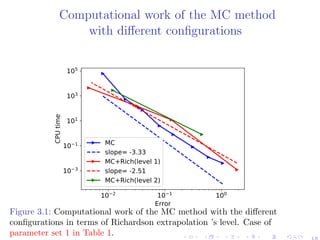


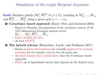
This document summarizes a research paper about using hierarchical deterministic quadrature methods for option pricing under the rough Bergomi model. It discusses the rough Bergomi model and challenges in pricing options under this model numerically. It then describes the methodology used, which involves analytic smoothing, adaptive sparse grids quadrature, quasi Monte Carlo, and coupling these with hierarchical representations and Richardson extrapolation. Several figures are included to illustrate the adaptive construction of sparse grids and simulation of the rough Bergomi dynamics.


![Ica group 3[1]](https://cdn.slidesharecdn.com/ss_thumbnails/icagroup31-191026172214-thumbnail.jpg?width=640&height=640&fit=bounds)