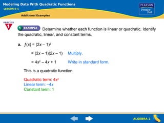
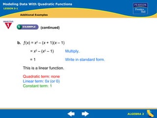
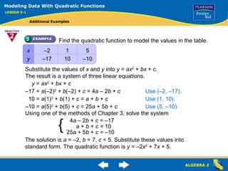
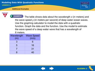
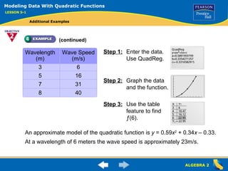
The document discusses identifying quadratic, linear, and constant terms in functions. It then provides examples of determining if functions are quadratic or linear and finding the vertex and axis of symmetry of quadratic functions. The document concludes by using a table of data to model a real-world scenario with a quadratic function.

1. Determine whether each function is linear or quadratic. Identify the quadratic, linear, and constant terms. a. ƒ ( x ) = (2 x – 1) 2 This is a quadratic function. Quadratic term: 4 x 2 Linear term: –4 x Constant term: 1 Modeling Data With Quadratic Functions LESSON 5-1 Additional Examples = (2 x – 1)(2 x – 1) Multiply. = 4 x 2 – 4 x + 1 Write in standard form.

2. (continued) b. ƒ ( x ) = x 2 – ( x + 1)( x – 1) This is a linear function. Quadratic term: none Linear term: 0 x (or 0) Constant term: 1 Modeling Data With Quadratic Functions LESSON 5-1 Additional Examples = x 2 – ( x 2 – 1) Multiply. = 1 Write in standard form.

3. Below is the graph of y = x 2 – 6 x + 11. Identify the vertex and the axis of symmetry. Identify points corresponding to P and Q . Modeling Data With Quadratic Functions LESSON 5-1 Additional Examples The vertex is (3, 2). The axis of symmetry is x = 3. P (1, 6) is two units to the left of the axis of symmetry. Corresponding point P (5, 6) is two units to the right of the axis of symmetry. Q (4, 3) is one unit to the right of the axis of symmetry. Corresponding point Q (2, 3) is one unit to the left of the axis of symmetry.

4. Find the quadratic function to model the values in the table. The solution is a = –2, b = 7, c = 5. Substitute these values into standard form. The quadratic function is y = –2 x 2 + 7 x + 5. Using one of the methods of Chapter 3, solve the system Modeling Data With Quadratic Functions LESSON 5-1 Additional Examples x y – 2 – 17 1 10 5 – 10 Substitute the values of x and y into y = ax 2 + bx + c . The result is a system of three linear equations. y = ax 2 + bx + c 4 a – 2 b + c = –17 a + b + c = 10 25 a + 5 b + c = –10 { – 17 = a (–2) 2 + b (–2) + c = 4 a – 2 b + c Use (–2, –17). 10 = a (1) 2 + b (1) + c = a + b + c Use (1, 10). – 10 = a (5) 2 + b (5) + c = 25 a + 5 b + c Use (5, –10).

5. The table shows data about the wavelength x (in meters) and the wave speed y (in meters per second) of deep water ocean waves. Use the graphing calculator to model the data with a quadratic function. Graph the data and the function. Use the model to estimate the wave speed of a deep water wave that has a wavelength of 6 meters. Wavelength (m) 3 5 7 8 Wave Speed (m/s) 6 16 31 40 Modeling Data With Quadratic Functions LESSON 5-1 Additional Examples

6. (continued) An approximate model of the quadratic function is y = 0.59 x 2 + 0.34 x – 0.33. At a wavelength of 6 meters the wave speed is approximately 23m/s. Modeling Data With Quadratic Functions LESSON 5-1 Additional Examples Wavelength (m) 3 5 7 8 Wave Speed (m/s) 6 16 31 40 Step 1: Enter the data. Use QuadReg. Step 2: Graph the data and the function. Step 3: Use the table feature to find ƒ (6).