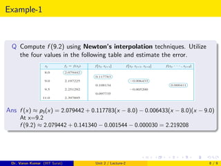
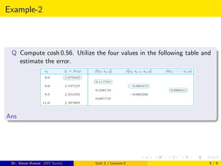
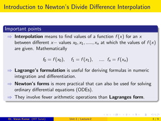
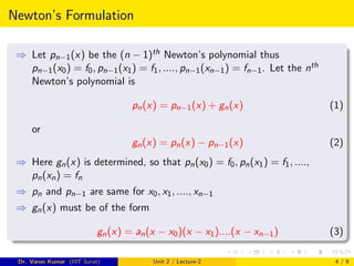
Newton’s Divided Difference Interpolation
Dr. Varun Kumar
Dr. Varun Kumar (IIIT Surat) Unit 2 / Lecture-2 1 / 9
Outlines
1 Introduction to Newton’s Divide Difference Interpolation
2 Example
Dr. Varun Kumar (IIIT Surat) Unit 2 / Lecture-2 2 / 9
Introduction to Newton’s Divide Difference Interpolation
Important points
⇒ Interpolation means to find values of a function f (x) for an x
between different x− values x0, x1, ....., xn at which the values of f (x)
are given. Mathematically
f0 = f (x0), f1 = f (x1), .... fn = f (xn)
⇒ Lagrange’s formulation is useful for deriving formulas in numeric
integration and differentiation.
⇒ Newton’s forms is more practical that can also be used for solving
ordinary differential equations (ODEs).
⇒ They involve fewer arithmetic operations than Lagranges form.
Dr. Varun Kumar (IIIT Surat) Unit 2 / Lecture-2 3 / 9
Newton’s Formulation
⇒ Let pn−1(x) be the (n − 1)th Newton’s polynomial thus
pn−1(x0) = f0, pn−1(x1) = f1, ...., pn−1(xn−1) = fn−1. Let the nth
Newton’s polynomial is
pn(x) = pn−1(x) + gn(x) (1)
or
gn(x) = pn(x) − pn−1(x) (2)
⇒ Here gn(x) is determined, so that pn(x0) = f0, pn(x1) = f1, ....,
pn(xn) = fn
⇒ pn and pn−1 are same for x0, x1, ...., xn−1
⇒ gn(x) must be of the form
gn(x) = an(x − x0)(x − x1)....(x − xn−1) (3)
Dr. Varun Kumar (IIIT Surat) Unit 2 / Lecture-2 4 / 9
Continued–
⇒ Using (3), let x = xn
an =
fn − pn−1(xn−1)
(xn − x0)(xn − x1)....(xn − xn−1)
⇒ We write ak instead of an and show that ak equals to the kth divided
difference, recursively.
a1 = f [x0, x1] =
f1 − f0
x1 − x0
a2 = f [x0, x1, x2] =
f [x1, x2] − f [x0, x1]
x2 − x0
ak = f [x0, ...., xk] =
f [x1, x2, .., xk] − f [x0, ..xk−1]
xk − x0
Dr. Varun Kumar (IIIT Surat) Unit 2 / Lecture-2 5 / 9
Continued–
⇒ If n = 1, then pn−1(xn) = p0(x1) = f0 because p0(x) is constant.
Hence from (3)
a1 =
f1 − p0(x1)
x1 − x0
=
f1 − f0
x1 − x0
= f [x0, x1]
⇒ Hence Newton’s interpolation for the first degree
p1(x) = f0 + (x − x0)f [x0, x1]
⇒ If n = 2, then pn−1(xn) = p1(x2). Hence from (3)
a2 =
f2 − p1(x2)
(x2 − x1)(x2 − x0)
=
f2 − f0 − (x2 − x0)f [x0, x1]
(x2 − x1)(x2 − x0)
= f [x0, x1, x2]
Dr. Varun Kumar (IIIT Surat) Unit 2 / Lecture-2 6 / 9
Continued–
⇒ We thus obtain the second Newton’s polynomial
p2(x) = f0 + (x − x0)f [x0, x1] + (x − x0)(x − x1)f [x0, x1, x2]
⇒ For n = k, we can write
pk(x) = pk−1(x) + (x − x0)(x − x1)....(x − xk−1)f [x0....xk]
⇒ The more generalized Newton’s divide and difference
interpolation formula can be expressed as
f (x)= f0 + (x − x0)f [x0, x1] + (x − x0)(x − x1)f [x0, x1, x2] + ...+
= (x − x0)(x − x1)....(x − xn−1)f [x0, ..., xn]
Dr. Varun Kumar (IIIT Surat) Unit 2 / Lecture-2 7 / 9
Example-1
Q Compute f (9.2) using Newton’s interpolation techniques. Utilize
the four values in the following table and estimate the error.
Ans f (x) ≈ p3(x) = 2.079442 + 0.117783(x − 8.0) − 0.006433(x − 8.0)(x − 9.0)
At x=9.2
f (9.2) ≈ 2.079442 + 0.141340 − 0.001544 − 0.000030 = 2.219208
Dr. Varun Kumar (IIIT Surat) Unit 2 / Lecture-2 8 / 9
Example-2
Q Compute cosh 0.56. Utilize the four values in the following table and
estimate the error.
Ans
Dr. Varun Kumar (IIIT Surat) Unit 2 / Lecture-2 9 / 9

Newton's Divide and Difference Interpolation

  • 1.
    Newton’s Divided DifferenceInterpolation Dr. Varun Kumar Dr. Varun Kumar (IIIT Surat) Unit 2 / Lecture-2 1 / 9
  • 2.
    Outlines 1 Introduction toNewton’s Divide Difference Interpolation 2 Example Dr. Varun Kumar (IIIT Surat) Unit 2 / Lecture-2 2 / 9
  • 3.
    Introduction to Newton’sDivide Difference Interpolation Important points ⇒ Interpolation means to find values of a function f (x) for an x between different x− values x0, x1, ....., xn at which the values of f (x) are given. Mathematically f0 = f (x0), f1 = f (x1), .... fn = f (xn) ⇒ Lagrange’s formulation is useful for deriving formulas in numeric integration and differentiation. ⇒ Newton’s forms is more practical that can also be used for solving ordinary differential equations (ODEs). ⇒ They involve fewer arithmetic operations than Lagranges form. Dr. Varun Kumar (IIIT Surat) Unit 2 / Lecture-2 3 / 9
  • 4.
    Newton’s Formulation ⇒ Letpn−1(x) be the (n − 1)th Newton’s polynomial thus pn−1(x0) = f0, pn−1(x1) = f1, ...., pn−1(xn−1) = fn−1. Let the nth Newton’s polynomial is pn(x) = pn−1(x) + gn(x) (1) or gn(x) = pn(x) − pn−1(x) (2) ⇒ Here gn(x) is determined, so that pn(x0) = f0, pn(x1) = f1, ...., pn(xn) = fn ⇒ pn and pn−1 are same for x0, x1, ...., xn−1 ⇒ gn(x) must be of the form gn(x) = an(x − x0)(x − x1)....(x − xn−1) (3) Dr. Varun Kumar (IIIT Surat) Unit 2 / Lecture-2 4 / 9
  • 5.
    Continued– ⇒ Using (3),let x = xn an = fn − pn−1(xn−1) (xn − x0)(xn − x1)....(xn − xn−1) ⇒ We write ak instead of an and show that ak equals to the kth divided difference, recursively. a1 = f [x0, x1] = f1 − f0 x1 − x0 a2 = f [x0, x1, x2] = f [x1, x2] − f [x0, x1] x2 − x0 ak = f [x0, ...., xk] = f [x1, x2, .., xk] − f [x0, ..xk−1] xk − x0 Dr. Varun Kumar (IIIT Surat) Unit 2 / Lecture-2 5 / 9
  • 6.
    Continued– ⇒ If n= 1, then pn−1(xn) = p0(x1) = f0 because p0(x) is constant. Hence from (3) a1 = f1 − p0(x1) x1 − x0 = f1 − f0 x1 − x0 = f [x0, x1] ⇒ Hence Newton’s interpolation for the first degree p1(x) = f0 + (x − x0)f [x0, x1] ⇒ If n = 2, then pn−1(xn) = p1(x2). Hence from (3) a2 = f2 − p1(x2) (x2 − x1)(x2 − x0) = f2 − f0 − (x2 − x0)f [x0, x1] (x2 − x1)(x2 − x0) = f [x0, x1, x2] Dr. Varun Kumar (IIIT Surat) Unit 2 / Lecture-2 6 / 9
  • 7.
    Continued– ⇒ We thusobtain the second Newton’s polynomial p2(x) = f0 + (x − x0)f [x0, x1] + (x − x0)(x − x1)f [x0, x1, x2] ⇒ For n = k, we can write pk(x) = pk−1(x) + (x − x0)(x − x1)....(x − xk−1)f [x0....xk] ⇒ The more generalized Newton’s divide and difference interpolation formula can be expressed as f (x)= f0 + (x − x0)f [x0, x1] + (x − x0)(x − x1)f [x0, x1, x2] + ...+ = (x − x0)(x − x1)....(x − xn−1)f [x0, ..., xn] Dr. Varun Kumar (IIIT Surat) Unit 2 / Lecture-2 7 / 9
  • 8.
    Example-1 Q Compute f(9.2) using Newton’s interpolation techniques. Utilize the four values in the following table and estimate the error. Ans f (x) ≈ p3(x) = 2.079442 + 0.117783(x − 8.0) − 0.006433(x − 8.0)(x − 9.0) At x=9.2 f (9.2) ≈ 2.079442 + 0.141340 − 0.001544 − 0.000030 = 2.219208 Dr. Varun Kumar (IIIT Surat) Unit 2 / Lecture-2 8 / 9
  • 9.
    Example-2 Q Compute cosh0.56. Utilize the four values in the following table and estimate the error. Ans Dr. Varun Kumar (IIIT Surat) Unit 2 / Lecture-2 9 / 9