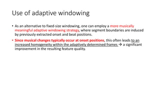
Downloaded 23 times


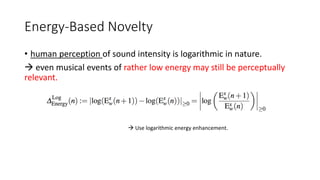
![Energy-Based Novelty
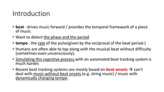
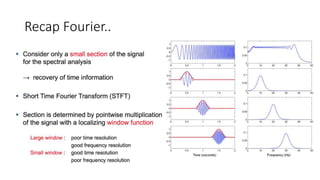
• Let‘s assume..
• w is a bell-shaped function centered at time zero.
• w(m) for m ∈ [−M : M] comprises the nonzero samples of w for some M ∈ N.
• local energy of x with regard to w is defined to be the function 𝐸 𝑤
𝑥 : Z → R given by for n ∈ Z
contains the energy of the signal x
multiplied with a window(bell-shaped) shifted by n samples](https://image.slidesharecdn.com/mpch6-170403153600/85/Fundamentals-of-music-processing-chapter-6-14-320.jpg)
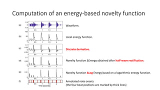

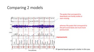
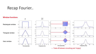
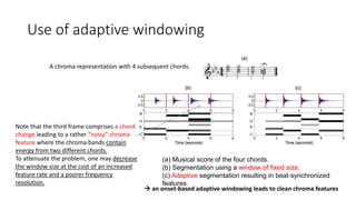
![Spectral-Based Novelty
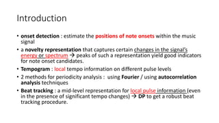
1) Convert the signal into a time–frequency representation
2) Capture changes in the frequency content.
let X be the discrete STFT of the DT-signal x :
(the sampling rate Fs= 1/T , the window length N of the discrete window w, the hop size
H.)
X(n,k) ∈ C (complex number)
: k-th Fourier coefficient for frequency index k ∈ [0 : K] and time frame n ∈ Z,
where K = N/2 is the frequency index corresponding to the Nyquist frequency.](https://image.slidesharecdn.com/mpch6-170403153600/85/Fundamentals-of-music-processing-chapter-6-23-320.jpg)


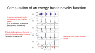
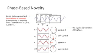
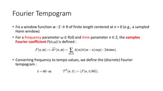
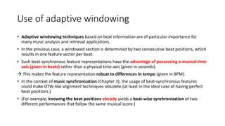
![Phase-Based Novelty
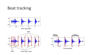
• Before, we only used the magnitude of the spectral coefficients, but now we use
the phase.
• let X(n,k) ∈ C be the complex-valued Fourier coefficient for frequency index k ∈ [0
: K] and time frame n ∈ Z.
• Using the polar coordinate representation,
• The phase φ(n,k) determines how the sinusoid of frequency Fcoef(k) = Fs · k/N
has to be shifted to best correlate with the windowed signal corresponding to
the nth frame.
complex coefficient phase](https://image.slidesharecdn.com/mpch6-170403153600/85/Fundamentals-of-music-processing-chapter-6-33-320.jpg)
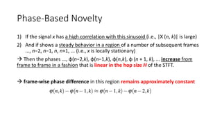

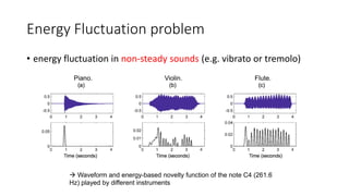
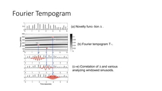
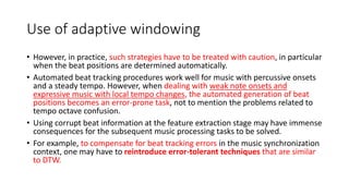
![Phase-Based Novelty
• So, a simultaneous disturbance of the values φ′′(n,k) for k ∈ [0 : K]
good indicator for note onsets.
• the phase-based novelty function ∆Phase :](https://image.slidesharecdn.com/mpch6-170403153600/85/Fundamentals-of-music-processing-chapter-6-37-320.jpg)
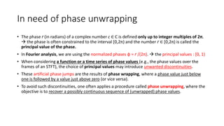
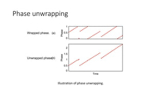
![Phase unwrapping
• Such a procedure, however, is in general not well defined since the original time series may possess “real”
discontinuities that are hard to distinguish from “artificial” phase jumps.
• In the onset detection context, phase jumps due to wrapping may occur when computing the
differences.(1st-order/2nd-order). In these cases, one needs to use an unwrapped version of the phase. As an
alternative, we introduce a principal argument function :
• A suitable integer value is added to or subtracted from the original phase difference yield a value in [−0.5,
0.5].
• Even though the principal argument function may cancel out large discontinuities in the phase differences,
this effect is attenuated since we consider the sum of differences over all frequency indices.](https://image.slidesharecdn.com/mpch6-170403153600/85/Fundamentals-of-music-processing-chapter-6-39-320.jpg)
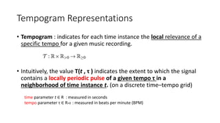
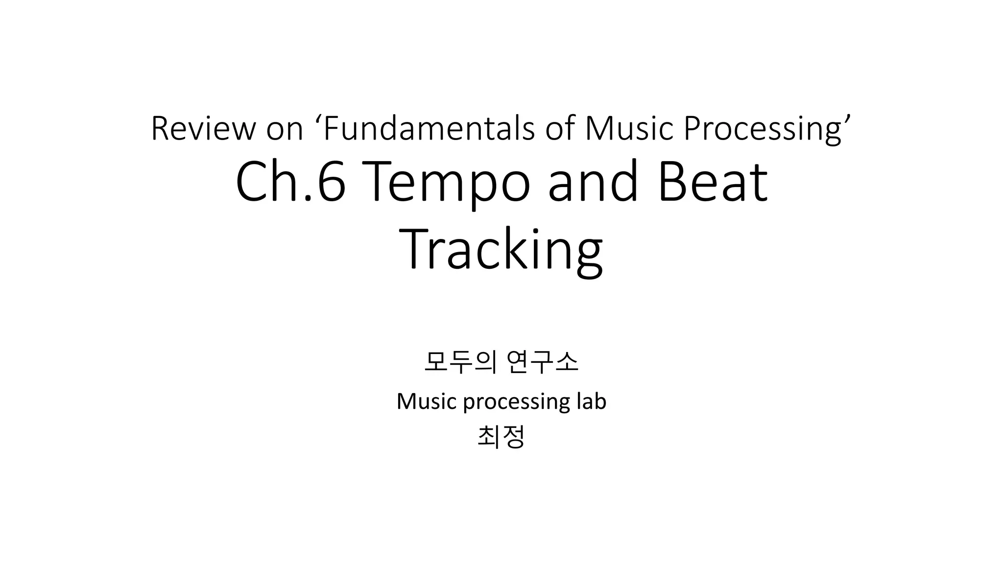
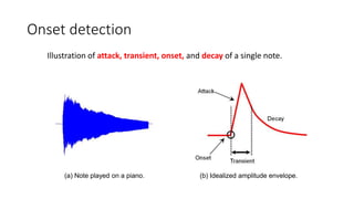
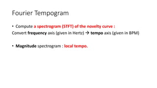
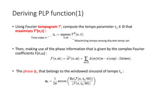
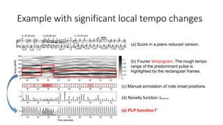
![Tempogram Representations
• the sampled time axis is given by [1 : N]. (we extend this axis to Z.)
• Θ⊂R > 0 : a finite set of tempi specified in BPM.
• a discrete tempogram is a function :](https://image.slidesharecdn.com/mpch6-170403153600/85/Fundamentals-of-music-processing-chapter-6-49-320.jpg)
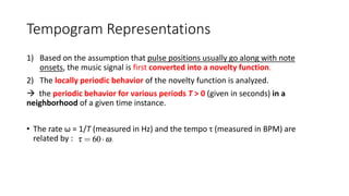
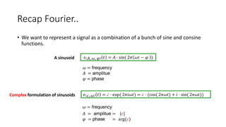

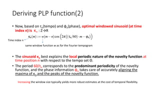
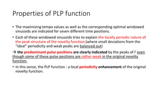
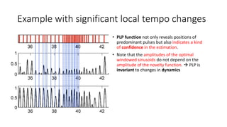
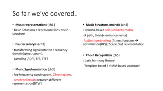
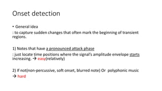
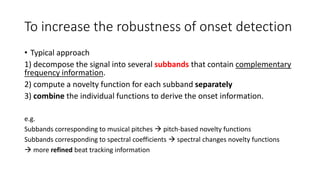
![Properties of PLP
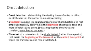
Beat level adjustment by tempo
range restriction based on a piano
recording.
Tempograms and PLP functions
(KS= 4 sec) are shown for various
sets Θ specifying the tempo range
used (given in BPM).
(a) Θ = [30 : 600] (full tempo range).
(b) Θ = [60 : 200] (tempo range
around quarter-note level).
(c) Θ = [200 : 340] (tempo range
around eighth-note level).
(d) Θ = [450 : 600] (tempo range
around sixteenth-note level).
Such switches in the pulse level can be avoided by constraining the tempo set Θ in the maximization.](https://image.slidesharecdn.com/mpch6-170403153600/85/Fundamentals-of-music-processing-chapter-6-85-320.jpg)

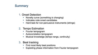
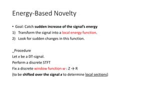
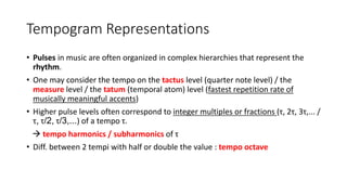
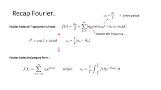
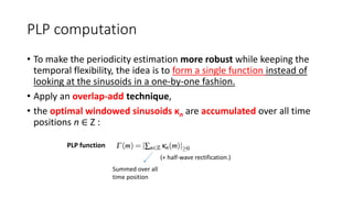
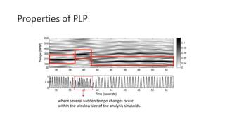
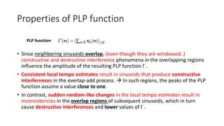
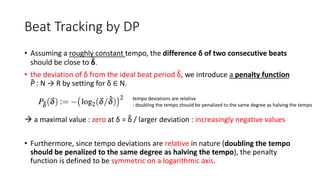
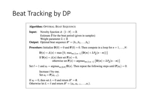
![Beat Tracking by DP
• Input :
1) a novelty function ∆ :[1:N]→R
2) a rough estimate τ ∈R>0 (global tempo)
(interval [1 : N] sampled time axis used for the novelty feature computation.)
• Rough tempo estimate τ :
manually or
from τ and the feature rate an estimate for the beat period δ.
: Maximum tempo from the time-averaged tempogram.](https://image.slidesharecdn.com/mpch6-170403153600/85/Fundamentals-of-music-processing-chapter-6-88-320.jpg)
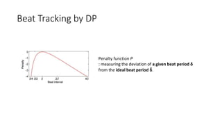
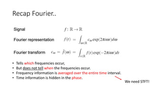
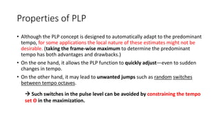
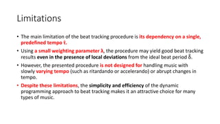
![Beat Tracking by DP
• For a given N ∈ N, let B = (b1,b2,...,bL) be a sequence of length L ∈ N0 consisting
of strictly monotonically increasing beat positions bl ∈ [1 : N] for l ∈ [1 : L].
beat sequence (beat sequence of length L = 0 is the empty sequence)
• let BN denote the set consisting of all possible beat sequences for a given
parameter N ∈ N.
• a score value S(B) : the quality of a beat sequence B ∈ BN
(positive values of the novelty function ∆ + negative values of the penalty function Pδ
)](https://image.slidesharecdn.com/mpch6-170403153600/85/Fundamentals-of-music-processing-chapter-6-91-320.jpg)
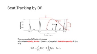
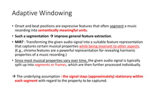
![Beat Tracking by DP
• Number of possible beat sequences is exponential in N dynamic programming.
• Let Bn
N ⊂ BN denote the set of all(possible) beat sequences that end in n ∈ [0 : N].
In other words, for a beat sequence B = (b1,b2,...,bL) ∈ Bn
N, we have bL = n. (in the case n = 0, the
only possible beat sequence is the empty one.)
• the maximal score S(B∗) for an optimal beat sequence B∗ is obtained by looking for the largest
value of D:
accumulated score : maximal score over all beat sequences ending with n ∈ [0 : N]](https://image.slidesharecdn.com/mpch6-170403153600/85/Fundamentals-of-music-processing-chapter-6-94-320.jpg)
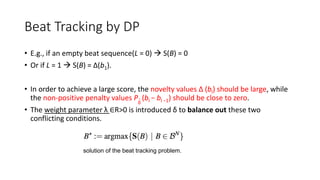
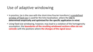
![Beat Tracking by DP
D(n) can be computed in an iterative fashion for n = 0,1,...,N
1) n = 0 : initializing the procedure
D(n) = 0
2) n > 0
- Assuming that we already know the values D(m) for m ∈ [0 : n − 1], we need to compute the value
D(n).
- B∗n = (b1,b2,...,bL) with bL = n : a score-maximizing beat sequence that yields D(n) = S(B∗n).
Though we may not know such a sequence explicitly, we know, at least, that the last beat bL = n
contributes with the novelty value ∆(n).](https://image.slidesharecdn.com/mpch6-170403153600/85/Fundamentals-of-music-processing-chapter-6-95-320.jpg)
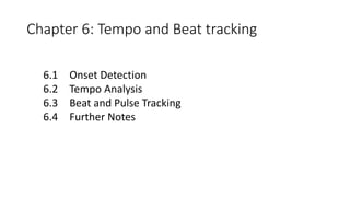
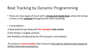
![Beat Tracking by DP
• The first case is L = 1, where one has a single beat and D(n) = ∆ (n). The second case is L > 1,
where one has a beat bL−1 ∈ [1 : n − 1] that precedes bL = n. Using S(B), the accumulated score
D(n) is obtained by :
• In other words, the optimal score D(n) :
• the sum of the novelty value ∆(n)
• the (weighted) penalty of the beat period δ = bL− bL−1
• the optimal score D(bL−1) of a beat sequence ending at bL−1
• Even though we do not know bL−1 explicitly so far, we have already computed all values D(m) for
m ∈ [0 : n − 1]. From this and by considering the two cases (L = 1 and L > 1), we obtain the
following recursion:
: accumulated score
?](https://image.slidesharecdn.com/mpch6-170403153600/85/Fundamentals-of-music-processing-chapter-6-96-320.jpg)
![Beat Tracking by DP
• Apply a backtracking procedure
• While calculating D(n), we additionally store the information on the maximization
process by means of a number P(n) ∈ [0 : n − 1].
In the case that the maximum is 0, we have L = 1 and there is no preceding beat.
Therefore, we set P(n) := 0.
Otherwise, one has L > 1, and there is a preceding beat. In this case we set](https://image.slidesharecdn.com/mpch6-170403153600/85/Fundamentals-of-music-processing-chapter-6-97-320.jpg)
![Beat Tracking by DP
• Here, the maximizing index n∗ ∈ [0 : N] determines the last beat bL = n∗ of an optimal
beat sequence B∗. (Only in the case n∗ = 0, there is no last beat and B∗ = 0.)
• The remaining beats of B∗ can then be obtained by backtracking using the predecessor
information supplied by P.
• In the case P(n∗) = 0, the backtracking is terminated and L = 1.
• bL−1 = P(bL) determines the beat preceding the last beat bL = n∗. This procedure is then
iterated to determine bL−2 = P(bL−1), bL−3 = P(bL−2), and so on, until the condition P(b1) =
0 terminates the backtracking.
• (Note that the length L is not known a priori and results from the backtracking.)
• Computing quadratic in N
n∗](https://image.slidesharecdn.com/mpch6-170403153600/85/Fundamentals-of-music-processing-chapter-6-98-320.jpg)

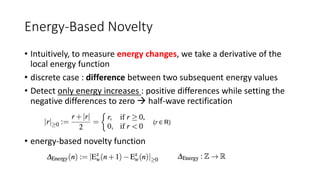
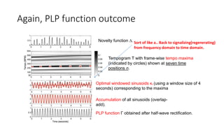
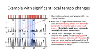
![Shortened window
• (new pararm for shortening window) λ ∈ R, 0 < λ < 1 : determines the size of the neighborhoods.
• s,t ∈ [1 : N] : the start and end positions of a given adaptive window
determine the start and end positions of the shortened windowing used for the
feature computation.
With this definition, the center of the adaptive window is preserved, while its
size is reduced by a factor λ relative to its original size (t − s)](https://image.slidesharecdn.com/mpch6-170403153600/85/Fundamentals-of-music-processing-chapter-6-109-320.jpg)

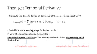
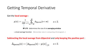
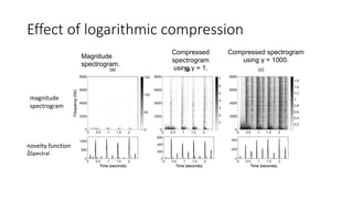
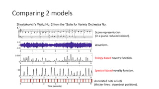
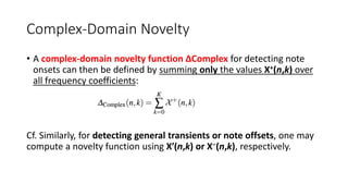
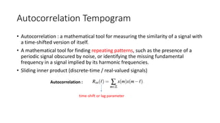
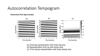
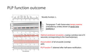
The document summarizes different techniques for tempo and beat tracking in music processing. It discusses onset detection methods like energy-based and spectral-based novelty functions to detect note onsets. It then covers tempo analysis using tempogram representations to capture local tempo characteristics. Beat tracking aims to determine the phase and period of the musical beat by considering onset detections and periodicity analysis using Fourier or autocorrelation techniques. Dynamic programming can be used to obtain a robust beat tracking procedure.


![[Tutorial] Computational Approaches to Melodic Analysis of Indian Art Music](https://cdn.slidesharecdn.com/ss_thumbnails/tutorialmelodicanalysis-170910111235-thumbnail.jpg?width=640&height=640&fit=bounds)


