Downloaded 305 times


![1. %xa(t)= exp(-10|t|)
2. %CTFT is given by Xa(F) =
[(2*10)/(10^2 + (2*pi*F)^2)]
3. %sampling xa(t) at Fs = 50
samples/sec
4. clear all
5. tmin = -1;
6. tmax = 1;
7. %Analog signal
8. t = tmin: 0.001: tmax;
9. xa = exp(-10*abs(t));
10. %Sampling
rate(sample/second)
11. Fs = 50;
12. %Sample period
13. Ts = 1/Fs;
14. %Discrete time signal
15. n = tmin/Ts:tmax/Ts;
16. x = exp(-10*abs(n*Ts));
17. %Display signal in time
domain
18. figure(1)
19. subplot(211)
20. plot(t,xa)
21. title('Analog and
Discrete Time Signals')
22. xlabel('time(sec)')
23. ylabel('Analog Signal
x(t)')
24. subplot(212)
25. stem(n,x)
26. xlabel('n')
27. ylabel('Discrete time
signal x(n)')
28. %Computing FT
29. %Analog frequency (Hz)
30. F = -100:0.1:100;
31. W = (2*pi*F);
32. %DT Frequency
(circles/sample)
33. f = F/Fs;
34. w = 2*pi*f;
35. %Analog spectrum for
CTFT
36. XaF = 2.*(10./(10^2+
W.^2));
37. %DTFT
38. XF = x * exp(-1i*n'*w);
39. %Display spectra in
frequency domain
40. figure(2)
41. subplot(311)
42. plot(F,abs(XaF))
43. title('spectra of
signals')
44. xlabel('Freq(circle/sec
)')
45. ylabel('Original
Xa(F)')
46. subplot(312)
47. plot(F,abs(XF))
48. xlabel('Freq(circle/sec
)')
49. ylabel('X(F/Fs)')
50. subplot(313)
51. plot(f,abs(XF))
52. xlabel('Freq(circle/sec
)')
53. ylabel('X(f)')
54. %Display spectra in the
fundamental range
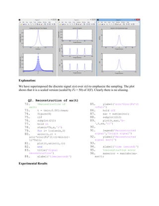
55. figure(3)
56. subplot(211)
57. plot(F,abs(XaF))
58. plot(F,abs(XF))
59. title('spectra in the
fundamental range')
60. xlabel('Freq(circle/sec
)')
61. ylabel('X(F/Fs)')
62. v = axis;
63. v(1:2) = [-Fs/2 Fs/2];
64. axis(v)
65. subplot(212)
66. plot(f,abs(XF))
67. xlabel('Freq(circle/sec
)')
68. ylabel('X(f)')
69. v = axis;
70. v(1:2) = [-1/2 1/2];
71. axis(v)
Experimental results](https://image.slidesharecdn.com/dspassignment1matlab-161012031335/85/DIGITAL-SIGNAL-PROCESSING-Sampling-and-Reconstruction-on-MATLAB-5-320.jpg)
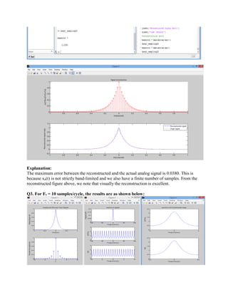

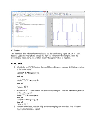


The document is a MATLAB assignment focused on the sampling and reconstruction of analog signals in the context of digital signal processing (DSP). It explains sampling principles, including the necessity of sampling above the Nyquist rate to avoid aliasing, and covers multiple interpolation methods for reconstruction. Experimental results demonstrate the effects of different sampling rates and provide MATLAB code for various scenarios, along with discussions on reconstruction errors and the importance of adhering to the sampling theorem.


![Digital Signal Processing[ECEG-3171]-Ch1_L05](https://cdn.slidesharecdn.com/ss_thumbnails/dspl5ch2-180427094424-thumbnail.jpg?width=640&height=640&fit=bounds)

![Introduction to Signal Processing Orfanidis [Solution Manual]](https://cdn.slidesharecdn.com/ss_thumbnails/51628783-solution-signal-processing-160422182740-thumbnail.jpg?width=640&height=640&fit=bounds)


![Digital Signal Processing[ECEG-3171]-Ch1_L06](https://cdn.slidesharecdn.com/ss_thumbnails/dspl6ch2-180427094424-thumbnail.jpg?width=640&height=640&fit=bounds)