Fourier Transforms of Discrete
Signals
Microlink IT College
ambawb
Sampling
• Continuous signals are digitized using digital computers
• When we sample, we calculate the value of the continuous
signal at discrete points
– How fast do we sample
– What is the value of each point
• Quantization determines the value of each samples value
ambawb
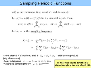
Sampling Periodic Functions
- Note that wb = Bandwidth, thus if then aliasing occurs
(signal overlaps)
-To avoid aliasing
-According sampling theory: To hear music up to 20KHz a CD
should sample at the rate of 44.1 KHz
ambawb
Discrete Time Fourier Transform
• In likely we only have access to finite amount of data
sequences (after sampling)
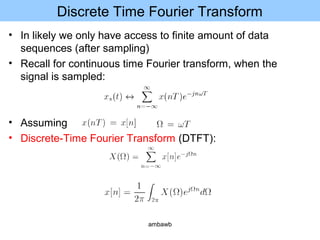
• Recall for continuous time Fourier transform, when the
signal is sampled:
• Assuming
• Discrete-Time Fourier Transform (DTFT):
ambawb
Discrete Time Fourier Transform
• Discrete-Time Fourier Transform (DTFT):
• A few points
– DTFT is periodic in frequency with period of 2π
– X[n] is a discrete signal
– DTFT allows us to find the spectrum of the discrete signal as viewed
from a window
ambawb
Example D
See map!
ambawb
Example of Convolution
• Convolution
– We can write x[n] (a periodic function) as an infinite sum of the
function xo[n] (a non-periodic function) shifted N units at a time
– This will result
– Thus
See map!
ambawb
Finding DTFT For periodic signals
• Starting with xo[n]
• DTFT of xo[n]
Example
ambawb
Example A & B
notes
notes
X[n]=a|n|
, 0 < a < 1.
ambawb
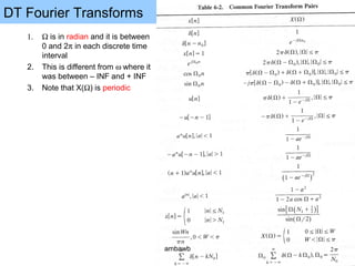
DT Fourier Transforms
1. Ω is in radian and it is between
0 and 2π in each discrete time
interval
2. This is different from ω where it
was between – INF and + INF
3. Note that X(Ω) is periodic
ambawb
Properties of DTFT
• Remember:
• For time scaling note that
m>1  Signal spreading
ambawb
Fourier Transform of Periodic Sequences
• Check the map~~~~~
See map!
ambawb
Discrete Fourier Transform
• We often do not have an infinite amount of data which is
required by DTFT
– For example in a computer we cannot calculate uncountable infinite
(continuum) of frequencies as required by DTFT
• Thus, we use DTF to look at finite segment of data
– We only observe the data through a window
– In this case the xo[n] is just a sampled data between n=0, n=N-1 (N
points)
ambawb
Discrete Fourier Transform
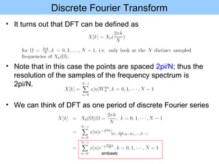
• It turns out that DFT can be defined as
• Note that in this case the points are spaced 2pi/N; thus the
resolution of the samples of the frequency spectrum is
2pi/N.
• We can think of DFT as one period of discrete Fourier series
ambawb
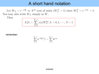
A short hand notation
remember:
ambawb
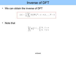
Inverse of DFT
• We can obtain the inverse of DFT
• Note that
ambawb
Using MATLAB to Calculate DFT
• Example:
– Assume N=4
– x[n]=[1,2,3,4]
– n=0,…,3
– Find X[k]; k=0,…,3
or
ambawb
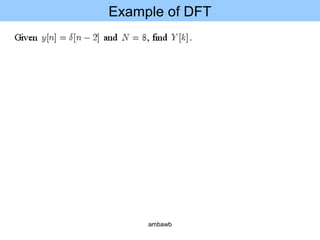
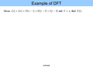
Example of DFT
• Find X[k]
– We know k=1,.., 7; N=8
ambawb
Example of DFT
ambawb
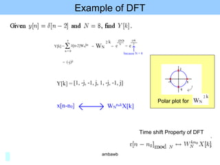
Example of DFT
Time shift Property of DFT
Polar plot for
ambawb
Example of DFT
ambawb
Example of DFT
Summation for X[k]
Using the shift property!
ambawb
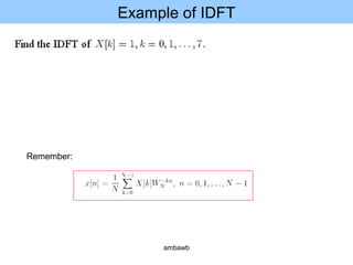
Example of IDFT
Remember:
ambawb
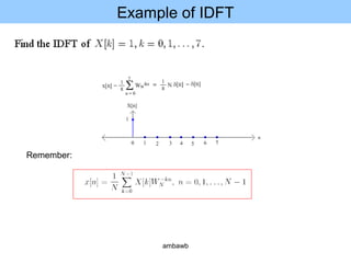
Example of IDFT
Remember:
ambawb
Fast Fourier Transform Algorithms
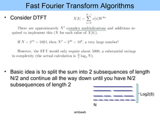
• Consider DTFT
• Basic idea is to split the sum into 2 subsequences of length
N/2 and continue all the way down until you have N/2
subsequences of length 2
Log2(8)
N
ambawb
Radix-2 FFT Algorithms - Two point FFT
• We assume N=2^m
– This is called Radix-2 FFT Algorithms
• Let’s take a simple example where only two points are given n=0, n=1; N=2
y0
y1
y0
Butterfly FFT
Advantage: Less
computationally
intensive: N/2.log(N)
Advantage: Less
computationally
intensive: N/2.log(N)
ambawb
General FFT Algorithm
• First break x[n] into even and odd
• Let n=2m for even and n=2m+1 for odd
• Even and odd parts are both DFT of a N/2 point
sequence
• Break up the size N/2 subsequent in half by letting
2mm
• The first subsequence here is the term x[0], x[4], …
• The second subsequent is x[2], x[6], …
1
1)2sin()2cos(
)]12[(]2[
2/
2
2/
2/
2/2/
2/
2/
2/
2
12/
0
2/
12/
0
2/
−=
=−−−==
==
=
++
−
+
−
=
−
=
∑∑
N
N
jN
N
m
N
N
N
m
N
Nm
N
mk
N
mk
N
N
m
mk
N
k
N
N
m
mk
N
W
jeW
WWWW
WW
mxWWmxW
πππ
ambawb
Example
1
1)2sin()2cos(
)]12[(]2[][
2/
2
2/
2/
2/2/
2/
2/
2/
2
12/
0
2/
12/
0
2/
−=
=−−−==
==
=
++=
−
+
−
=
−
=
∑∑
N
N
jN
N
m
N
N
N
m
N
Nm
N
mk
N
mk
N
N
m
mk
N
k
N
N
m
mk
N
W
jeW
WWWW
WW
mxWWmxWkX
πππ
Let’s take a simple example where only two points are given n=0, n=1; N=2
]1[]0[]1[]0[)]1[(]0[]1[
]1[]0[)]1[(]0[]0[
1
1
0
0
1.0
1
1
1
0
0
1.0
1
0
0
0.0
1
0
1
0
0
0.0
1
xxxWxxWWxWkX
xxxWWxWkX
mm
mm
−=+=+==
+=+==
∑∑
∑∑
==
==
Same result
ambawb
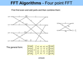
FFT Algorithms - Four point FFT
First find even and odd parts and then combine them:
The general form:
ambawb
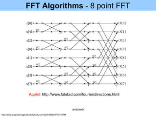
FFT Algorithms - 8 point FFT
http://www.engineeringproductivitytools.com/stuff/T0001/PT07.HTM
Applet: http://www.falstad.com/fourier/directions.html
ambawb
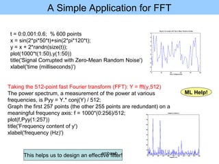
A Simple Application for FFT
t = 0:0.001:0.6; % 600 points
x = sin(2*pi*50*t)+sin(2*pi*120*t);
y = x + 2*randn(size(t));
plot(1000*t(1:50),y(1:50))
title('Signal Corrupted with Zero-Mean Random Noise')
xlabel('time (milliseconds)')
Taking the 512-point fast Fourier transform (FFT): Y = fft(y,512)
The power spectrum, a measurement of the power at various
frequencies, is Pyy = Y.* conj(Y) / 512;
Graph the first 257 points (the other 255 points are redundant) on a
meaningful frequency axis: f = 1000*(0:256)/512;
plot(f,Pyy(1:257))
title('Frequency content of y')
xlabel('frequency (Hz)')
This helps us to design an effective filter!
ML Help!
ambawb
Example
• Express the DFT of the 9-point {x[0], …,x[9]} in terms of the
DFTs of 3-point sequences {x[0],x[3],x[6]}, {x[1],x[4],x[7]},
and {x[2],x[5],x[8]}.
ambawb
References
• Read Schaum’s Outlines: Chapter 6
• Do Chapter 12 problems: 19, 20, 26, 5, 7
ambawb

Fft

  • 1.
    Fourier Transforms ofDiscrete Signals Microlink IT College ambawb
  • 2.
    Sampling • Continuous signalsare digitized using digital computers • When we sample, we calculate the value of the continuous signal at discrete points – How fast do we sample – What is the value of each point • Quantization determines the value of each samples value ambawb
  • 3.
    Sampling Periodic Functions -Note that wb = Bandwidth, thus if then aliasing occurs (signal overlaps) -To avoid aliasing -According sampling theory: To hear music up to 20KHz a CD should sample at the rate of 44.1 KHz ambawb
  • 4.
    Discrete Time FourierTransform • In likely we only have access to finite amount of data sequences (after sampling) • Recall for continuous time Fourier transform, when the signal is sampled: • Assuming • Discrete-Time Fourier Transform (DTFT): ambawb
  • 5.
    Discrete Time FourierTransform • Discrete-Time Fourier Transform (DTFT): • A few points – DTFT is periodic in frequency with period of 2π – X[n] is a discrete signal – DTFT allows us to find the spectrum of the discrete signal as viewed from a window ambawb
  • 6.
  • 7.
    Example of Convolution •Convolution – We can write x[n] (a periodic function) as an infinite sum of the function xo[n] (a non-periodic function) shifted N units at a time – This will result – Thus See map! ambawb
  • 8.
    Finding DTFT Forperiodic signals • Starting with xo[n] • DTFT of xo[n] Example ambawb
  • 9.
    Example A &B notes notes X[n]=a|n| , 0 < a < 1. ambawb
  • 10.
    DT Fourier Transforms 1.Ω is in radian and it is between 0 and 2π in each discrete time interval 2. This is different from ω where it was between – INF and + INF 3. Note that X(Ω) is periodic ambawb
  • 11.
    Properties of DTFT •Remember: • For time scaling note that m>1  Signal spreading ambawb
  • 12.
    Fourier Transform ofPeriodic Sequences • Check the map~~~~~ See map! ambawb
  • 13.
    Discrete Fourier Transform •We often do not have an infinite amount of data which is required by DTFT – For example in a computer we cannot calculate uncountable infinite (continuum) of frequencies as required by DTFT • Thus, we use DTF to look at finite segment of data – We only observe the data through a window – In this case the xo[n] is just a sampled data between n=0, n=N-1 (N points) ambawb
  • 14.
    Discrete Fourier Transform •It turns out that DFT can be defined as • Note that in this case the points are spaced 2pi/N; thus the resolution of the samples of the frequency spectrum is 2pi/N. • We can think of DFT as one period of discrete Fourier series ambawb
  • 15.
    A short handnotation remember: ambawb
  • 16.
    Inverse of DFT •We can obtain the inverse of DFT • Note that ambawb
  • 17.
    Using MATLAB toCalculate DFT • Example: – Assume N=4 – x[n]=[1,2,3,4] – n=0,…,3 – Find X[k]; k=0,…,3 or ambawb
  • 18.
    Example of DFT •Find X[k] – We know k=1,.., 7; N=8 ambawb
  • 19.
  • 20.
    Example of DFT Timeshift Property of DFT Polar plot for ambawb
  • 21.
  • 22.
    Example of DFT Summationfor X[k] Using the shift property! ambawb
  • 23.
  • 24.
  • 25.
    Fast Fourier TransformAlgorithms • Consider DTFT • Basic idea is to split the sum into 2 subsequences of length N/2 and continue all the way down until you have N/2 subsequences of length 2 Log2(8) N ambawb
  • 26.
    Radix-2 FFT Algorithms- Two point FFT • We assume N=2^m – This is called Radix-2 FFT Algorithms • Let’s take a simple example where only two points are given n=0, n=1; N=2 y0 y1 y0 Butterfly FFT Advantage: Less computationally intensive: N/2.log(N) Advantage: Less computationally intensive: N/2.log(N) ambawb
  • 27.
    General FFT Algorithm •First break x[n] into even and odd • Let n=2m for even and n=2m+1 for odd • Even and odd parts are both DFT of a N/2 point sequence • Break up the size N/2 subsequent in half by letting 2mm • The first subsequence here is the term x[0], x[4], … • The second subsequent is x[2], x[6], … 1 1)2sin()2cos( )]12[(]2[ 2/ 2 2/ 2/ 2/2/ 2/ 2/ 2/ 2 12/ 0 2/ 12/ 0 2/ −= =−−−== == = ++ − + − = − = ∑∑ N N jN N m N N N m N Nm N mk N mk N N m mk N k N N m mk N W jeW WWWW WW mxWWmxW πππ ambawb
  • 28.
    Example 1 1)2sin()2cos( )]12[(]2[][ 2/ 2 2/ 2/ 2/2/ 2/ 2/ 2/ 2 12/ 0 2/ 12/ 0 2/ −= =−−−== == = ++= − + − = − = ∑∑ N N jN N m N N N m N Nm N mk N mk N N m mk N k N N m mk N W jeW WWWW WW mxWWmxWkX πππ Let’s take asimple example where only two points are given n=0, n=1; N=2 ]1[]0[]1[]0[)]1[(]0[]1[ ]1[]0[)]1[(]0[]0[ 1 1 0 0 1.0 1 1 1 0 0 1.0 1 0 0 0.0 1 0 1 0 0 0.0 1 xxxWxxWWxWkX xxxWWxWkX mm mm −=+=+== +=+== ∑∑ ∑∑ == == Same result ambawb
  • 29.
    FFT Algorithms -Four point FFT First find even and odd parts and then combine them: The general form: ambawb
  • 30.
    FFT Algorithms -8 point FFT http://www.engineeringproductivitytools.com/stuff/T0001/PT07.HTM Applet: http://www.falstad.com/fourier/directions.html ambawb
  • 31.
    A Simple Applicationfor FFT t = 0:0.001:0.6; % 600 points x = sin(2*pi*50*t)+sin(2*pi*120*t); y = x + 2*randn(size(t)); plot(1000*t(1:50),y(1:50)) title('Signal Corrupted with Zero-Mean Random Noise') xlabel('time (milliseconds)') Taking the 512-point fast Fourier transform (FFT): Y = fft(y,512) The power spectrum, a measurement of the power at various frequencies, is Pyy = Y.* conj(Y) / 512; Graph the first 257 points (the other 255 points are redundant) on a meaningful frequency axis: f = 1000*(0:256)/512; plot(f,Pyy(1:257)) title('Frequency content of y') xlabel('frequency (Hz)') This helps us to design an effective filter! ML Help! ambawb
  • 32.
    Example • Express theDFT of the 9-point {x[0], …,x[9]} in terms of the DFTs of 3-point sequences {x[0],x[3],x[6]}, {x[1],x[4],x[7]}, and {x[2],x[5],x[8]}. ambawb
  • 33.
    References • Read Schaum’sOutlines: Chapter 6 • Do Chapter 12 problems: 19, 20, 26, 5, 7 ambawb