SlideShare a Scribd company logo
1 of 18
Download to read offline
Chapter 2
p
Digitization
Digitization
of
Analog Signals
Contents
Contents
1. Introduction
2. Waveform coding
3. Subband and transform coding
g
4. Source coding (Analysis-by-Synthesis - AbS)
5 Vocoders (Parametric coders)
5. Vocoders (Parametric coders)
6. Concluding remarks
2
1. Introduction
Digitizing or digitization: the representation of an
object, image, sound, document or a (analog)
signal by a discrete set of its points or samples that
could receive limited values The result is
could receive limited values. The result is
called digital representation or, more specifically, a
digital image, for the object, and digital form, for the
signal. Strictly speaking, digitizing means simply
f
capturing an analog signal in digital form.
T ê ô Độ lậ ủ Chí h hủ
Tuyên ngôn Độc lập của Chính phủ
Lâm thời nước Việt Nam Dân chủ
Cộng hoà, ngày 2-9-1945. (Văn bản
scan). Bảo tàng Lịch sử Quốc gia.
Format
3
1. Introduction
Digital info.
E d
Transmit
Pulse
d l t
S l Q ti
Format
Textual
info.
Analog
source
Encode modulate
Sample Quantize
Channel
Pulse
waveforms
Bit stream
Format
Analog
info.
Demodulate/
Detect
Receive
Low-pass
filter
Decode
wave o s
Format
Textual
Analog
info.
i k Textual
info.
Digital info.
sink
4
1. Introduction
 Speech coding is the process of obtaining a compact representation of voice
signals for efficient transmission over band-limited wired and wireless channels
d/ t
Speech coding
and/or storage.
 Speech coders are lossy, i.e. the decoded signal is different from the original.
 The goal in speech coding is to minimize the distortion at a given bit rate, or
i i i th bit t t h i di t ti
 Categories:
 Waveform coding
 Subband and transform coding
minimize the bit rate to reach a given distortion.
LPC-AS: Linear Prediction
g
 Source (analysis-by-synthesis) coding
 Vocoders
Characteristics of Standardized Speech Coding
Algorithms in Each of Four Broad Categories
LPC-AS: Linear Prediction
Coding - Analysis-by-Synthesis
Speech Coder Class Rates (kbps) Complexity Standardized Applications
Waveform coders 16-64 Low Landline telephone
Subband coders 12-256 Medium Teleconferencing, audio
LPC AS 4 8 16 High Digital cellular
LPC-AS 4.8-16 High Digital cellular
LPC vocoder 2.0-4.8 High Satellite telephony, military
5
R t BW St d d St d d
A Representative Sample of Speech Coding Standards
Application
Rate
(kbps)
BW
(kHz)
Standards
Organization
Standard
Number
Algorithm Year
Landline
telephone
64
16-40
16 40
3.4
3.4
3 4
ITU
ITU
ITU
G.711
G.726
G 727
μ-law or A-law PCM
ADPCM
ADPCM
1988
1990
1990
16-40 3.4 ITU G.727 ADPCM 1990
Tele
conferencing
48-64
16
7
3.4
ITU
ITU
G.722
G.728
Split-band ADPCM
Low-delay CELP
1988
1992
Digital cellular 13
12 2
3.4
3 4
ETSI
ETSI
Full-rate
EFR
RPE-LTP
ACELP
1992
1997
12.2
7.9
6.5
8.0
4 75 12 2
3.4
3.4
3.4
3.4
3 4
ETSI
TIA
ETSI
ITU
ETSI
EFR
IS-54
Half-rate
G.729
AMR
ACELP
VSELP
VSELP
ACELP
ACELP
1997
1990
1995
1996
1998
4.75-12.2
1-8
3.4
3.4
ETSI
CDMA-TIA
AMR
IS-96
ACELP
QCELP
1998
1993
Multimedia 5.3-6.3
2.0-18.2
3.4
3.4-7.5
ITU
ISO
G.723.1
MPEG-4
MPLPC, CELP
HVXC, CELP
1996
1998
S t llit 4 15 3 4 INMARSAT M IMBE 1991
Satellite
telephony
4.15
3.6
3.4
3.4
INMARSAT
INMARSAT
M
Mini-M
IMBE
AMBE
1991
1995
Secure
communi-
ti
2.4
2.4
4 8
3.4
3.4
3 4
DDVPC
DDVPC
DDVPC
FS1015
MELP
FS1016
LPC-10e
MELP
CELP
1984
1996
1989
cations 4.8
16-32
3.4
3.4
DDVPC
DDVPC
FS1016
CVSD
CELP
CVSD
1989
1987
6
2 1 B i f Si l Di iti ti
2. WAVEFORM CODING
2.1. Basis of Signal Digitization
2.1.1.1 The sampling theorem
2.1.1 The Nyquist Sampling
 Simply referred to of other names such
as Shannon sampling theorem,
Nyquist-Shannon-Kotelnikov,
p g
y
Whittaker-Shannon-Kotelnikov,
Whittaker-Nyquist-Kotelnikov-
Shannon, WKS, etc., as well as the
Cardinal Theorem of Interpolation
Theory.
 To be a fundamental result in the field
of information theory, in particular
Hypothetical spectrum of a band-limited
signal as a function of frequency
y, p
telecommunications and signal
processing.
“Exact reconstruction of a continuous-time baseband signal from its
g
samples is possible if the signal is band-limited and the sampling
frequency is greater than twice the signal bandwidth.”
7
2.1.1.1 The sampling theorem …
 The assumptions necessary to prove the theorem form a mathematical model
that is only an idealized approximation of any real-world situation. The
conclusion, that perfect reconstruction is possible, is mathematically correct
for the model but only an approximation for actual signals and actual
for the model, but only an approximation for actual signals and actual
sampling techniques.
 The signal x(t) is band-limited to a one-sided baseband bandwidth if:
X(f ) 0 f ll | f | > B
X(f ) = 0 for all | f | > B.
 Then the sufficient condition for exact reconstructability from samples at a
uniform sampling rate (in samples per unit time)
f > 2B i l tl B < f /2
fs > 2B, or equivalently, B < fs/2.
 2B is called the Nyquist rate and is a property of the bandlimited signal, while
fs/2 is called the Nyquist frequency and is a property of this sampling system.
 The time inter al bet een s ccessi e samples is referred to as the sampling
 The time interval between successive samples is referred to as the sampling
interval T ≡ 1/fs and the samples of x(t) are denoted by x[n] ≡ x(nT), n Î 
(intergers).
 Including two processes: sampling and reconstruction
 Including two processes: sampling and reconstruction.
8
2.1.1.1 The sampling theorem …
 Sampling process: The continuous signal varying over time is sampled by
measuring the signal's value every T units of time (or space), which is called
the sampling interval.
 Reconstruction process of the original signal is an interpolation process that
mathematically defines a continuous-time signal x(t) from the discrete samples
x[n] and at times in between the sample instants nT by the following
procedure: Each sample value is multiplied by the sinc function scaled so that
the zero-crossings of the sinc function occur at the sampling instants and that
the sinc function's central point is shifted to the time of that sample, nT. All of
these shifted and scaled functions are then added together to recover the
original signal. The scaled and time-shifted sinc functions are continuous
making the sum of these also continuous, so the result of this operation is a
continuous signal. This procedure is represented by the Whittaker-Shannon
g p p y
interpolation formula:
 
   
 
sin ( / ) sin ( / )
( ) ( )
s s s s
f t n f f t n f
x t a a f x t dt
 

  
 
 
   
( ) ( )
( / ) ( / )
n n s
n s s s s
x t a a f x t dt
f t n f f t n f
 
 
 
 
9
2.1.1.1 The sampling theorem …
10
2.1.1.1 The sampling theorem …
Time domain Frequency domain
)
(
)
(
)
( t
x
t
x
t
xs 
  )
(
)
(
)
( f
X
f
X
f
Xs 
 
|
)
(
| f
X
)
(t
x
|
)
(
| f
X
)
(t
x
|
)
(
| f
Xs
)
(t
xs
|
)
(
| f
s
11
2.1.1.2. Aliasing effect
LP filter
Nyquist rate
aliasing
 Original file (sampling frequency 44 1 kHz stereo)
Demo!!!
 Original file (sampling frequency 44.1 kHz, stereo)
 Downsampling to 11.025 kHz without prefiltering (mono)
 Downsampling to 11.025 kHz with prefiltering (mono) 12
2.1.1.2. Aliasing effect …
 Examples of reconstruction problems due to aliasing
p p g
13
 I l li
2.1.1.3. How to sampling?
 Impulse sampling
 Natural sampling
 Sample and hold
14
2.1.1.3. How to sampling? …
Impulse sampling
15
2.1.1.3. How to sampling? …
Natural sampling
16
2.1.1.3. How to sampling? …
Sample and hold
17
2.1.1.4. Bandpass (under) sampling
 B i id
What are about
the problems with
 Basic idea
the problems with
sampling bandpass
signals?
18
 Resulting conditions needed for aliasing-free BP sampling
Allowed (white) and forbidden (shaded) sampling frequencies 19
 Example: Consider FM radio (in Vietnam) operating on the frequency band [fL
÷ fH] = [88 ÷ 108] MHz. The bandwidth W = fH - fL = 20 MHz. The sampling
di i
conditions:
Therefore, k can be 1, 2, 3, 4, or 5. k = 5 gives the lowest sampling frequencies
i t l 43 2 f 44 MH ( i f d li ) I thi th
     
   
1 5.4 = 108 MHz / 20 MHz
k
interval 43.2 < fs < 44 MHz (a scenario of undersampling). In this case, the
signal spectrum fits between 2 and 2.5 times the sampling rate (higher than
86.4 ÷ 88 MHz but lower than 108 ÷ 110 MHz). Stringent antialias filtering!!!
A lower value of k will also lead to a useful sampling rate For example
A lower value of k will also lead to a useful sampling rate. For example,
using k = 4, the FM band spectrum fits easily between 1.5 and 2.0 times the
sampling rate, for a sampling rate near 56 MHz (multiples of the Nyquist
frequency being 28, 56, 84, 112, etc.). Simpler antialias filtering!!!
20
2.1.1.5. Generalization: Under/critical/over sampling
(Lấy mẫu dưới/tới/quá hạn) … may be overloaded!!!
2.1.2. Quantisation
 A lit d ti i M i l f
 Amplitude quantizing: Mapping samples of a
continuous amplitude waveform to a finite set of
amplitudes.
 Uniform (linear) quantizing:
Out
( ) q g
In
ed
Quantize
values
21
2.1.2. Quantisation …
 Example:
111 3.1867
Amplitude x(t)
 Example:
( T ) l d l
quant. levels
111 3.1867
110 2.2762
101 1.3657
x(nTs): sampled values
boundaries
100 0.4552
011 -0.4552
( T ) ti d l
boundaries
011 0.4552
010 -1.3657
001 -2.2762
Ts: sampling time
xq(nTs): quantized values
00 . 76
000 -3.1867
t
PCM
codeword 110 110 111 110 100 010 011 100 100 011PCM sequence
22
 Quantizing (roundoff) error: The difference between the input and output
2.1.2. Quantisation …
 Quantizing (roundoff) error: The difference between the input and output
of a quantizer:
 Bernard Widrow showed that if the input random variable has a band-
limited characteristic function then the input distribution can be recovered
)
(
)
(
ˆ
)
( t
x
t
x
t
e 

limited characteristic function, then the input distribution can be recovered
from the quantized-output distribution, and the quantization noise density
is uniform.
M d l f i i i
P f i i i
)
(t
x )
(
ˆ t
x
Model of quantizing noise
)
(x
q
y 
Quantizer
Process of quantizing noise
)
( )
(
)
(t
e
)
(t
x )
(
ˆ t
x
AGC
x
)
(
q
y
ˆ
( ) ( ) ( )
e t x t x t
 
+
x
( )
e t
23
( )
2.1.2. Quantisation …
 Quantizing error types:
 Granular or linear errors happen for inputs within the dynamic range of
quantizer
 Saturation errors happen for inputs outside the dynamic range of quantizer
o Saturation errors are larger than linear errors
o Saturation errors can be avoided by proper tuning of AGC
 Quantization noise variance (linear):
 Average quantization noise power
2
2 q
 
 Signal peak power
12
 
2 2
2
p
L q
V 
M l b d !!!
 Signal power to average quantization noise power
4
p
2
2
3
p
V
S
L
 
 
  Matlab demo!!!
24
2
3
q
L
N 
 
 
 
Statistical of speech amplitudes
1.0
nction
2.1.2. Quantisation …
Statistical of speech amplitudes
0.5
ty
density
fun
 For a fixed, uniform quantizer, an
input signal with an amplitude
0.0
1.0 2.0 3 0
Probabilit
less than full load will have a
lower SQNR than a signal whose
amplitude occupies the full
dynamic range of the quantizer
 Such a variation in performance (SQNR) as a function of quantizer input
signal amplitude is particularly detrimental for speech, since low amplitude
1.0 3.0
Normalized magnitude of speech signal
dynamic range of the quantizer
(but without overload).
g p p y p , p
signals can be very important perceptually.
 In speech, weak signals are more frequent than strong ones. Speech is
generally stated to have a gamma or Laplacian probability density, which is
hi hl k d b t
highly peaked about zero.
 Using equal step sizes (uniform quantizer) gives low SQNR for weak signals
and high SQNR for strong signals.
 Adjusting the step size of the quantizer by taking into account the speech
statistics improves the SNR for the input range.
25
2.1.2. Quantisation …
Uniform vesus non-uniform quantization
 Uniform (linear) quantizing:
 No assumption about amplitude statistics and correlation properties of the
No assumption about amplitude statistics and correlation properties of the
input.
 Not using the user-related specifications.
 Robust to small changes in input statistic by not finely tuned to a specific set
g p y y p
of input parameters.
 Simply implemented.
 Application of linear quantizer: Signal processing, graphic and display
applications, process control applications.
 Non-uniform quantizing:
 Using the input statistics to tune quantizer parameters.
 Larger SNR than uniform quantizing with same number of levels.
 Non-uniform intervals in the dynamic range with same quantization noise
variance.
A li ti f if ti C l d f h
 Application of non-uniform quantizer: Commonly used for speech.
26
N if ti ti
2.1.2. Quantisation …
Non-uniform quantization
 It is done by uniformly quantizing the “compressed” signal.
 At the receiver, an inverse compression characteristic, called “expansion” is
l d t id i l di t ti
employed to avoid signal distortion.
Compression + expansion companding
Compression expansion companding
)
(x
C
y  x̂
)
(t
y
)
(t
x )
(
ˆ t
y )
(
ˆ t
x
)
(
y x
x ŷ
Compressing Quantizing
Channel
Expanding
T itt R i
Channel
Transmitter Receiver
27
2.2. Pulse-Code Modulation - PCM
 A digital representation of an analog signal where
the magnitude of the signal is sampled regularly
at uniform intervals, then quantized to a series of
symbols in a digital (usually binary) code
symbols in a digital (usually binary) code.
 Has been used in digital telephone systems since
1940s and is also the standard form for digital
audio in computers and the compact disc.
p p
 Laid the foundation for today’s digital
transmission.
 Applications: T/E-carrier, Audio CD, DVD, Blu-ray,
pp y
HDMI, WAV file, …
 4-step processing:
 Band-limited filtering
S li
Ralph Miller – former
technical staff of Bell Labs
in the 1940s
2 2 1 Band limited (antialias) filtering
 Sampling
 Quantizing
 Coding
in the 1940s.
The inventor of PCM.
2.2.1. Band-limited (antialias) filtering
 Voice signal is frequency constrained around 4 kHz by a lowpass filter.
28
2.2.2. Sampling (Time discretization)
 fs = 8 Kilo-samples/sec or Ts = 125 μs.
µ-law algorithm
s p s μ
2.2.3. Quantisation (Amplitude discretization)
 The µ-law algorithm: A companding algorithm, primarily used in the digital
telecommunication systems of North America and Japan.
 Algorithm types: Two forms - analog version, and quantized digital version.
 Continuous: For a given input x, the equation for μ-law encoding is
where μ = 255 (8 bits) in the North American and Japanese standards.
μ-law expansion is then given by the inverse equation:
μ p g y q
 Discrete: Defined in ITU-T Recommendation G 711 Piece-wise linearly
 Discrete: Defined in ITU-T Recommendation G.711. Piece-wise linearly
approximated by 15 cords/segments.
29
A l l ith
2.2.3. Quantisation…
A-law algorithm
 Standard companding algorithm, used in European digital communications
systems to optimize, i.e., modify, the dynamic range of an analog signal for
digitizing
digitizing.
 Continuous: For a given input x, the equation for A-law encoding is as
follows,
where A is the compression parameter. In Europe, A = 87.7; the value
where A is the compression parameter. In Europe, A 87.7; the value
87.6 is also used.
A-law expansion is given by the inverse function,
 Discrete: Defined in ITU T Recommendation G 711 Piece wise linearly
 Discrete: Defined in ITU-T Recommendation G.711. Piece-wise linearly
approximated by 13 cords/segments
30
2.2.3. Quantisation…
15-segment µ-law
13-segment A-law
Discrete forms of non-uniform quantization
31
Quantized μ-law algorithm
14 bit binary linear input code 8 bit compressed code
 μ-law
2.2.4. Coding
14 bit binary linear input code 8 bit compressed code
+8159 to +4063 in 16 intervals of 256 1000ABCD
+4062 to +2015 in 16 intervals of 128 1001ABCD
+2014 to +991 in 16 intervals of 64 1010ABCD
μ
encoding thus
takes a 14-bit
signed linear
audio sample
+990 to +479 in 16 intervals of 32 1011ABCD
+478 to +223 in 16 intervals of 16 1100ABCD
+222 to +95 in 16 intervals of 8 1101ABCD
audio sample
as input and
converts it to
an 8 bit value
+94 to +31 in 16 intervals of 4 1110ABCD
+30 to +1 in 15 intervals of 2 1111ABCD
0 11111111
as follows:
PXYZABCD
 A bias of 33 is
−1 01111111
−31 to −2 in 15 intervals of 2 0111ABCD
−95 to −32 in 16 intervals of 4 0110ABCD
 A bias of 33 is
added to the
absolute input
value enabling
th d i t −223 to −96 in 16 intervals of 8 0101ABCD
−479 to −224 in 16 intervals of 16 0100ABCD
−991 to −480 in 16 intervals of 32 0011ABCD
2015 t 992 i 16 i t l f 64 0010ABCD
the endpoints
of each chord
to become
powers of two,
−2015 to −992 in 16 intervals of 64 0010ABCD
−4063 to −2016 in 16 intervals of 128 0001ABCD
−8159 to −4064 in 16 intervals of 256 0000ABCD
p ,
also reducing
max to 8159.
32
Quantized A-law algorithm
2.2.4. Coding…
Q g
13 bit binary linear input code 8 bit compressed code
+4096 to +2048 in 16 intervals of 128 1111ABCD
+2047 to +1024 in 16 intervals of 64 1110ABCD
 A-law
encoding
thus takes a
13-bit
+1023 to +512 in 16 intervals of 32 1101ABCD
+511 to +256 in 16 intervals of 16 1100ABCD
+255 to +128 in 16 intervals of 8 1011ABCD
13-bit
signed linear
audio
sample as
+127 to +64 in 16 intervals of 4 1010ABCD
+63 to +32 in 16 intervals of 2 1001ABCD
+31 to 0 in 16 intervals of 2 1000ABCD
input and
converts it to
an 8 bit
value as
−31 to −1 in 16 intervals of 2 0000ABCD
−63 to −32 in 16 intervals of 2 0001ABCD
−127 to −64 in 16 intervals of 4 0010ABCD
value as
follows:
−255 to −128 in 16 intervals of 8 0011ABCD
−511 to −256 in 16 intervals of 16 0100ABCD
−1023 to −512 in 16 intervals of 32 0101ABCD
2047 t 1024 i 16 i t l f 64 0110ABCD
−2047 to −1024 in 16 intervals of 64 0110ABCD
−4096 to −2048 in 16 intervals of 128 0111ABCD
33
Companding of μ-law and A-law algorithms
2.2.4. Coding…
Companding of μ-law and A-law algorithms
dBm0 - Power in dBm measured at a zero transmission level point
dBFS - dB relative to full scale (ex: 50% of peak power → -3 dBFS) 34
2.2.4. Coding…
 PCM signals is considered as a part of international connection.
 Quantisation noise must guarantee the performance of existing analog
routes.
 As in referencing network, for 1 link (S/N)q ≥ 22 dB with the average
dynamic range of voice from -25 to -5 dBm. The total referencing route
includes 14 links, adding 10log14 = 11.46 dB on the budget. So, (S/N)qTotal
= 33 46 dB
33.46 dB.
 This needs a 7-bit coder. Providing other degradation requires 8-bit coder.
 The code word: PXYZABCD.
 Finally before transmission the entire codeword is inverted since low
 Finally, before transmission, the entire codeword is inverted, since low
amplitude signals tend to be more numerous than large amplitude signals.
Consequently, inverting the bits increases the density of positive pulses on
the transmission line, which improves the hardware performance.
p p
 The μ-law algorithm provides a slightly larger dynamic range than the A-
law at the cost of worse proportional distortion for small signals.
 By convention, A-law is used for an international connection if at least one
y
country uses it.
35
2.3. Differential Pulse-Code Modulation - DPCM
m(t)
 Basic idea: PCM tries to represent
sample amplitudes → wasting
“resource” when adjacent samples
quite resemble one another
t
quite resemble one another.
Encoding the differences
between sample amplitudes is
more efficient → DPCM
 DPCM: A procedure of converting an analog into a digital signal in which an
analog signal is sampled and then the difference between the actual sample
value and its predicted value is quantized and then encoded forming a digital
l P di t d l i b d i l l
value. Predicted value is based on previous sample or samples.
 Most source signals show significant correlation between successive samples
so encoding using redundancy in sample values results in lower bit rate.
 R li ti f thi b i t i b d t h i di ti t
 Realization of this basic concept is based on a technique predicting current
sample value based upon previous sample(s) and encoding the difference
between actual value of sample and predicted value (prediction error).
 A form of predictive coding DPCM compression depends on the prediction
 A form of predictive coding. DPCM compression depends on the prediction
technique, well-conducted prediction techniques → good compression rates.
36
 Usually a linear predictor is used (linear predictive coding):
 Delta Modulation: 1-bit predictor
37
 A predictor can be realised with a tapped delay line to form a transversal filter.
 Delay line: “hangs onto" (delays) past samples
 Tapped: “tap into" line to pick up the desired signals
 The an are the tap gains, calculated according to some “best fit" algorithm
(e g minimum mean squared error)
(e.g., minimum mean squared error)
( )
x n
( )
( )
p
x n
38
 Small signal
variation of
variation of
DPCM
compared to
PCM means
l d d
less coded
bits needed.
 Also, the
signal
signal
statistics
improved.
39
 Signal distortions due to intraframe DPCM coding
 Granular noise: random noise in flat areas of the picture, waveform
Granular noise: random noise in flat areas of the picture, waveform
 Edge busyness: jittery appearance of edges (for video)
 Slope overload: blur of high-contrast edges,
Moire patterns in periodic tructures.
40
41
2.4. Adaptive DPCM - ADPCM
 Voice signal is not a strictly stationary but quasi-stationary process,
namely, its variance and autocorrelation slowly varies by time.
 Fixed stepsize uniform quantization might not result in quantization noise
p q g q
power of constant q2/12.
 Adaptively change the quantizing step size to maintain quantization noise
power constant (vector quantization method). Typically, the adaptation to
signal statistics in ADPCM consists simply of an adaptive scale factor
before quantizing the difference in the DPCM encoder.
 Adaptively change the predictor (tap gains an) to reduce predictive signal
distortions (vector prediction method)
distortions (vector prediction method).
 Resulting in coded bit rate of 16, 24, 32, 40 Kbps.
42
ITU-T ADPCM speech
codec standard
G.726 ADPCM encoder
43
G.726 ADPCM
decoder
44
3. SUBBAND AND TRANSFORM CODING
3 1 P i i l
3.1. Principles
 An analysis filterbank is first used to filter the signal into a number of frequency
bands and then bits are allocated to each band by a certain criterion.
 H b d tl f id b d di t hi h bit t h d
 Has been used mostly for wideband medium to high bit rate speech coders
and for audio coding.
 For example, in G.722, ADPCM speech coding occurs within two subbands,
and bit allocation is set to achieve 7 kHz audio coding at rates of 64 kbps or
and bit allocation is set to achieve 7-kHz audio coding at rates of 64 kbps or
less.
 A speech production model
is not used, ensuring
robustness to speech in the
presence of background
noise, and to non-speech
Hi h lit
sources. High-quality
compression can be
achieved by incorporating
masking properties of the
g p p
human auditory system.
45
 Not widely used for speech coding today, but it is expected that new
standards for wideband coding and rate-adaptive schemes will be based
sta da ds o deba d cod g a d ate adapt e sc e es be based
on subband coding or a hybrid technique that includes subband coding.
This is because subband coders are more easily scalable in bit rate than
standard CELP techniques, an issue which will become more critical for
high quality speech and audio transmission over wireless communication
high-quality speech and audio transmission over wireless communication
channels and the Internet, allowing the system to seamlessly adapt to
changes in both the transmission environment and network congestion.
3.2. Example: MPEG-1 Layer 3 (mp3)
46
4. SOURCE CODING
4.1. Speech Production Model
 Speech is generated by pumping
air from the lung through the
g g
vocal tract consisting of throat,
nose, mouth, palate, tongue,
teeth and lips.
Lax vocal
Nasal
cavity
Velum
Nasal
sound
output
cords - Open
for breathing
Vocal
Folds/
Cords
Pharyngeal
cavity
Tongue
Oral
cavity
output
Oral
Lungs
Trachea
hump sound
output
T d l Lungs
Tensed vocal
cords - Ready
to vibrate
47
 Voiced sounds: The
4.2. Voice/Voiceless Sounds
 Voiced sounds: The
tense vocal chords are
vibrating and the airflow
gets modulated. The
oscillation frequency of
the vocal chords is called
'pitch'. The vocal tract
colours the spectrum of
voiced
voiceless
colours the spectrum of
the pulsating air flow in a
sound-typical manner.
 Voiceless sounds: The
vocal chords are loose
and white-noise-like
turbulences are formed at
bottlenecks in the vocal
tract. The remaining vocal
tract colours the
turbulating airflow more
or less depending on the
position of the bottleneck.
Demo! 48
4.3. Formants
 One major property of
speech is its correlation, i.e.
successive samples of a
speech signal are similar
Vowel /a/ in short term
speech signal are similar.
 The short-term correlation
of successive speech
samples has consequences
for the short-term spectral
envelopes (< 10 ms).
 These spectral envelopes have a few local maxima, the so called 'formants'
which correspond to resonance frequencies of the human vocal tract. Speech
consists of a succession of sounds, the so-called phonemes. While speaking,
humans continuously change the setting of their vocal tract in order to produce
different resonance frequencies (formants) and therefore different sounds
different resonance frequencies (formants) and therefore different sounds.
 This (short-term) correlation can be used to estimate the current speech
sample from past samples. This estimation is called 'prediction'. Because the
prediction is done by a linear combination of (past) speech samples, it is called
'linear prediction'. The difference between the original and the estimated signal
is called 'prediction error signal'.
49
Vowel /a/: Spectral
estimations of original
signal (green), predicted
signal with 10-th order
short-term predictor (red)
and frequency response
of a 10-th order speech
model filter based on the
predictor coefficients
(blue). Four formants can
easily be identified.
 Ideally, all correlation is removed, i.e. the error signal is white noise. Only the
error signal is conveyed to the receiver: It has less redundancy, therefore
each bit carries more information. In other words: With less bits, we can
transport the same amount of information i e have the same speech quality
transport the same amount of information, i.e. have the same speech quality.
 The calculation of the prediction error signal corresponds to a linear filtering of
the original speech signal: The speech signal is the filter input, and the error
signal is the output. Main component of this filter is the (short-term) predictor.
signal is the output. Main component of this filter is the (short term) predictor.
The goal of the filter is to 'whiten' the speech signal, i.e. to filter out the
formants. That is why this filter is also called an 'inverse formant filter'.
50
 While speaking, the formants
continuously change → the short-
term correlation also changes and
the predictor must be adapted to the
these changes. Thus, the predictor
and the prediction error filter are
LPC Filter
and the prediction error filter are
adaptive filters whose parameters
must be continuously estimated from
the speech signal.
4.4. Pitch
 Voiced sounds as e.g. vowels have a periodic structure, i.e. their signal form
repeats itself after some milliseconds the so-called pitch period T Its
repeats itself after some milliseconds, the so called pitch period Tp. Its
reciprocal value fp = 1/Tp is called pitch frequency. So there is also correlation
between distant samples in voiced sounds.
 This long-term correlation is exploited for bit-rate reduction with a so-called
g p
long-term predictor (also called pitch predictor).
 Also the pitch frequency is no constant. Female speakers have higher pitch
than male speakers. The pitch frequency varies in a speaker-typical manner.
V i l d t d t h i di t t t ll d
Voice-less sounds as consonants do not have a periodic structure at all, and
mixed sounds with voice-less and voiced components also exist.
51
 Thus, also the pitch predictor must be implemented as an adaptive filter,
and the pitch period and the pitch gain must be continuously estimated
from the speech signal.
Vowel /a/ in long term
52
4.5. Spectrogram 0.3
“ee” “ee” “oh”
“oh”
 A useful representation of the
speech signal, showing the signal's
power distribution with respect to 0
0.1
0.2
plitude
ee ee oh
oh
time and frequency.
 The idea is to calculate the (short-
term) power spectral densities (this
i th d f
-0.2
-0.1
Amp
gives the power and frequency
information) of successive (this gives
the time information) fragments of
the signal. 3500
4000
0 5 10 15 20
-0.3
g
 Usually, the time is printed on the x-
scale of a spectrogram and the
frequency on the y-scale. The power 2000
2500
3000
ency
(Hz)
is coded in the color, for example
red means high power and blue low
power.
500
1000
1500
Freque
53
0
5 10 15 20
Time
4.6. Adaptive Predictive Coding
 Only the parameters of the inverse formant filter and the inverse pitch filter
plus the error signal are transmitted to the receiver. The receiver constructs
the inverse filters, i.e. a pitch filter and a formant filter, and reconstructs the
speech signal by inverse filtering of the error signal. This coding structure is
known as ‘Adaptive Predictive Coding’ - APC.
 APC is the basis for a variety of so-called waveform speech codecs which try
to preserve the waveform of the speech signal. The idea is not to convey the
p p g y
error signal completely: Only an equivalent version is transferred, or a version
carrying the main information. Thus we are saving bits.
54
4.7. RELP, MPE & RPE
 B b d R id l E it d Li P di ti (BB RELP) O l l
 Baseband Residual Excited Linear Prediction (BB-RELP): Only a low
pass-filtered version of the error signal (also called residual) is conveyed to
the receiver. The low pass-filtered version of the error signal can be down
sampled and fewer samples have to be transmitted. The decoder must
p p
somehow regenerate the missing spectral components, this is done by
simply repeating the spectral baseband information in the spectral domain (a
number of zeros = down sampling factor are padded in the time domain
between each sample)
between each sample).
 Multi-Pulse Excited Linear Prediction (MPE-LPC): The residual is
substituted by a small number of impulses (all other samples are set to
zero). Typically, 40 samples are replaced by 4 to 6 samples whose positions
and values are determined one after the other by minimizing the mean
square error (MSE) between the original and the synthesized speech signal.
 Regular-Pulse Excited Linear Prediction (RPE-LPC): This is similar to
MPE, but the pulses have a fixed distance. Only the position of the first pulse
must be transferred to the receiver. The pulse amplitudes can be found by
solving a linear equations. The GSM Full-Rate Codec is a mixture of an RPE
and a BB-RELP codec: The down sampling factor is three and the down
and a BB RELP codec: The down sampling factor is three, and the down
sampled excitation signal with the highest energy is chosen.
55
4.8. CELP – Codebook Excited Linear Prediction
 Modern algorithms (used in GSM, UMTS, LTE) have a limited storage of
potential prediction error signals (the stochastic codebook), and the index of
the best-fitting signal is transferred to the receiver → few bis transmitted.
 In the coder, each prediction error signal is already vocal-tract filtered and the
th th i d h i l i d t th i i l h i l b
thus synthesized speech signal is compared to the original speech signal by
applying an error measure, e.g. the MSE → 'analysis-by-synthesis'. Thus, a
vector quantization of the original speech segment is performed.
 The decoder has the same codebook available and can retrieve the best-
 The decoder has the same codebook available and can retrieve the best
fitting error signal with the index.
CELP P i i l
CELP Principle:
Analysis-by-
Synthesis. The best
codebook vector is
codebook vector is
determined and
afterwards the
corresponding best
i l i
gain value is
calculated.
56
 This scheme results in low bit rates but the speech quality is inferior:
Although intelligible, the codec sounds artificial and lacks naturalness
because voiced (periodic) speech frames are no good reproduced.
 Improvement can be done by performing an APC-like pitch analysis first.
The calculated LTP delay and LTP gain values are used for inducing a pitch
t t i t th t h ti d b k t i t th l i b
structure into the stochastic codebook vectors prior to the analysis-by-
synthesis. This idea is realized in the below scheme.
4.8.1. Open-Loop CELP
Open-Loop CELP Principle:
Analysis-by-Synthesis. The
decoder is fully included in the
coder Main part of the structure
coder. Main part of the structure
resembles an APC decoder.
57
4.8.2. Closed-Loop CELP
 The LTP analysis can also be included into the Analysis-by-Synthesis resulting
y y y y g
in an even better reproduction of voiced frames, especially for small LTP delay
values which are typical for female speakers → ‘Closed-loop’ CELP.
 This is the basis for state-of-the-art speech codecs as ITU-T G.729, ETSI GSM
Enhanced Fullrate Codec (EFR) etc works!
Enhanced Fullrate Codec (EFR) etc. works!
Closed-Loop
CELP Principle:
CELP Principle:
LTP included in
Analysis-by-
Synthesis.
58
4.8.3. Improving CELP's Speech Quality
The CELP codecs described here so far still do not sound good enough. Many
g g y
ideas resulted in a considerable improvement of the speech quality:
 The stochastic codebooks were trained with real speech material (instead of
simply white Gaussian noise).
 More complex error measures were introduced: Very typical is an error
weighting filter which is applied to the error signal before calculating the MSE:
Thus, the perceptual error is minimized according to psychoacoustic results.
f
 Another idea is to use more than one stochastic codebook in order to further
minimize the remaining error.
 'Fractional' delays can improve the pitch regeneration. An oversampling filter
is used to calculate intermediate samples of the past excitation signal of the
vocal-tract filter, and the delay value is thus no more restricted to a multiple of
the sampling period.
 Better quantization techniques for the parameter values use the available bit
rate more efficiently. Vector quantization of LPC coefficients or pitch
parameters is often found. Also, other representations for the LPC coefficients
improve their coding: E.g. Line Spectral Frequencies allow a representation of
10 LPC ffi i t ith l 28 bit
10 LPC coefficients with only 28 bits.
 Post-filters in the decoder can slightly improve the perceived speech quality.
59
 The analysis-by-synthesis is computationally very expensive → reduce the
4.8.4. CELP Implementation Considerations
e a a ys s by sy t es s s co putat o a y e y e pe s e educe t e
complexity (in terms of MIPs and MFLOPs). Most of the ideas concern the
stochastic codebook: By using special structures, the computational cost of the
vocal-tract filtering can be greatly simplified:
 Unity Magnitude Codebook: The optimal stochastic excitation signal can also
be searched in the frequency domain. If the Discrete Fourier Transforms of the
codebook vectors all have the same magnitude and differ only in phase, the
minimization procedure is greatly simplified
minimization procedure is greatly simplified.
 Vector-Sum CELP Codecs (VSELP) as e.g. the North American IS-54 have
only a few base vector, and all other stochastic vectors are derived by a linear
combination of these base vectors. Because the vocal-tract filter is a linear, only
y
the base vectors must be actually filtered, and the filtered stochastic vectors are
calculated by a linear combination of the filtered base vectors.
 Algebraic (structured) CELP Codecs (ACELP) as ITU-T G.729 and EFR use
d b k E h t h l f l ≠ 0 d th l
a sparse codebook: Each vector has only a few samples ≠ 0, and these samples
only have values of -1 and +1 (resolving memory shortage & complexity
problems). The properties of the codebook vectors can be optimized for the
current speech segment by applying a signal-adaptive filtering. The search for
p g y pp y g g p g
the optimal excitation can be efficiently performed in the excitation domain after
inverse vocal-tract filtering of the original speech signal.
60
The most popular codebook structure is the interleaved pulse permutation code,
in which, codevector consists of a set of interleaved permutation codes
containing only few non-zero elements: pi = i + jd, j = 0, 1,…, 2M − 1, where pi is
the pulse position, i is the pulse number, and d is the interleaving depth. The
integer M is the number of bits describing the pulse positions.
Example, interleaving depth d = 5, max
number of pulses/tracks = 5, number of
bits to represent the pulse positions
M = 3 → p = i + j5 where i = 0 1 2 3 4
Track(i) Pulse positions (pi)
0 p0: 0, 5, 10, 15, 20, 25, 30, 35
1 p1: 1, 6, 11, 16, 21, 26, 31, 36
2 p2: 2, 7, 12, 17, 22, 27, 32, 37
M = 3 → pi = i + j5, where i = 0,1,2,3,4
and j = 0,1,2,…,7.
For a given value of i, the set {pi} is known as ‘track,’ and the value of j defines
2 p2: 2, 7, 12, 17, 22, 27, 32, 37
3 p3: 3, 8, 13, 18, 23, 28, 33, 38
4 p4: 4, 9, 14, 19, 24, 29, 34, 39
g {pi} j
the pulse position. From the codebook structure shown in the above table, the
codevector, x(n), is given by,
4
( ) ( - ), 0,1,...,39,
i i
x n n p n
 
 

where δ(n) is the unit impulse, αi are the pulse amplitudes (±1) and pi are the
pulse positions. In particular, the codebook vector, x(n), is computed by placing
the 5 unit pulses at the determined locations p multiplied with their signs (±1)
0
( ) ( ), , ,..., 9,
i i
i
p
 


the 5 unit pulses at the determined locations, pi, multiplied with their signs (±1) .
The pulse position indices and the signs are encoded and transmitted.
Note that the algebraic codebooks do not require any storage! 61
ACELP map
62
4.9. Adaptive Multi-Rate Codec - AMR
 3G & 4G utilize the AMR codec. AMR offers several bitrates and can thus be
adapted to the current channel conditions. AMR is nothing special, it is just an
ACELP codec as described above. Different parameter settings lead to
different speech qualities and bitrates
different speech qualities and bitrates.
 ETSI adopted ACELP for GSM telephony operating at multiple rates: 12.2,
10.2, 7.95, 6.7, 5.9, 5.15, and 5.75 kb/s. The bit rate is adjusted according to
the traffic conditions.
 The Adaptive Multi-Rate WideBand (AMR-WB) is an ITU-T wideband standard
that has been jointly standardized with 3GPP, and it operates at rates 23.85,
23.05, 19.85, 18.25, 15.85, 14.25, 12.65, 8.85 and 6.6 kbps. The higher rates
provide better quality where background noise is stronger.
 The other two important speech coding standards are the Variable Rate
Multimode WideBand (VMR-WB, adopted by 3GPP2) with the source coding
t lli th bit t f ti ( t f 1 1/2 1/4 1/8 di t
controlling the bit rates of operation (rates of 1,1/2,1/4,1/8 corresponding to
13.3, 6.2, 2.7 and 1 kbps) and the extended AMR-WB (AMR-WB+) addressing
mixed speech and audio content, delivering high quality audio even at low bit
rates.
63
Reflection
coefficients coded as
4.10. GSM coder
Short term
LPC
analysis
(1) ( )
coefficients coded as
Log. - Area Ratios
(36 bits/20 ms)
RPE parameters
Input Pre-
processing
signal
Short term
analysis
filter
+
RPE grid
selection
and coding
(1) (2)
(3)
-
p
(47 bits/5 ms)
(13 pulses)
Long term
analysis
filter
+
RPE grid
decoding and
positioning
(4) (5)
13 Kbps RPE-LTP coder
(GSM 06.10 version
LTP
analysis
LTP parameters
(9 bits/5 ms)
(
8.1.1 Release 1999)
To
radio
subsystem
(1) Short term residual
(2) Long term residual (40 samples)
(3) Short term residual estimate (40 samples)
(4) Reconstructed short term residual (40 samples)
(5) Quantized long term residual (40 samples)
subsystem
( ) g ( p )
Simplified block diagram of the RPE – LTP encoder 64
13 Kbps RPE-LTP coder
(GSM 06.10 version 8.1.1 Release 1999)
4.10. GSM coder
Reflection coefficients coded
as Log. - Area Ratios
(36 bits/20 ms)
RPE grid
decoding and
positioning
+
Short term
synthesis
filter
Post-
processing
Output
signal
positioning
RPE
parameters
(47 bits/5 ms)
filter
Long term
synthesis
filter
g signal
(13 pulses)
LTP
parameters
(9 bits/5 ms)
From
radio
Simplified block diagram of the RPE - LTP decoder
subsystem
65
4.11. Extended Adaptive Multi-Rate - Wideband (AMR-WB+) codec
3GPP TS 26.290 V11.0.0 (2012-09)
HF signals folded in
0-Fs/4 kHz band
HF encoding
HF parameters
Input signal
L
LHF
RHF HF parameters
preprocesing
Input signal
R
Mono
LF parameters
HF encoding
MLF
RHF
mode
MHF
Input signal
HF parameters
preprocesing
and analysis
filterbank
ACELP/TCX
encoding
LF parameters
MUX
MLF
Stereo
parameters
LLF
MLF
g
M
Down
Mixing
(L,R)
to
(M,S)
Stereo
encoding
parameters
RLF
SLF
Mono operation
LF signals folded in
0-Fs/4 kHz band
AMR-WB+ - Extended Adaptive Multi-Rate Wideband
ACELP - Algebraic Code Excited Linear Prediction
High-level structure of AMR-WB+ encoder
g
TCX - Transform coded excitation (transform-based core-coder)
66
4.11. Extended Adaptive Multi-Rate - Wideband (AMR-WB+) codec
3GPP TS 26.290 V11.0.0 (2012-09)
HF parameters
HF decoding
LHF
LHF
HF parameters
HF signals folded in
0-Fs/4 kHz band
RHF
HF decoding
mode
RHF
MHF
Output signal
L
synthesis
filterbank and
postprocesing
Mono
LF parameters
DEMUX
ACELP/TCX
decoding
MLF
MHF
Output signal
R
Output signal
M
Stereo
parameters
Stereo
d di
LLF
RLF
decoding RLF
Mono operation AMR-WB+ - Extended Adaptive Multi-Rate Wideband
ACELP - Algebraic Code Excited Linear Prediction
TCX T f d d it ti (t f b d d )
High-level structure of AMR-WB+ decoder
TCX - Transform coded excitation (transform-based core-coder)
67
5. LPC Vocoders
 In practice all sounds have a mixed excitation which means that the excitation
 In practice, all sounds have a mixed excitation, which means that the excitation
consists of voiced and unvoiced portions. Of course, the relation of these
portions varies strongly with the sound being generated.
 An (over) simplification can be made in the sound production model by 'hard'
( ) p p y
switch between voiced and unvoiced excitation. Thus the excitation signal is
not transmitted at all but only some parameters describing it, e.g. its power.
Such an algorithm produces really artificial speech and is known as a 'Vocoder'
(Voice Coder)
(Voice Coder).
68
 This codec contains a simple classifier which decides whether the current
frame is a silence, voiceless or voiced frame: The signal level determines if it
is a silence frame or not, and if it is non-silence, the average zero-crossing
rate determines if it is voiceless or voiced (in voiceless frames, there are
more zero-crossings)
more zero crossings).
 The classifier result is feeded into a state-machine which takes the final
decision whether the frame shall be treated as silence, voiced or voiceless
(the idea is to smooth out changes from voiced/voiceless to silence).
( g )
 Mixed voiced/voiceless excitations are not supported by this implementation.
 In voiceless frames, only the mean signal amplitude and the predictor
coefficients are calculated and conveyed to the decoder.
y
 In voiced frames, also the pitch lag is estimated (with a very simple block
autocorrelation approach) and conveyed.
 The decoder creates an excitation signal from the silence (just zeroes),
g (j )
voiceless (just random noise) and voiced (just 1-pulses in a distance
corresponding to the current estimated pitch lag) information and filters it
with the adaptive vocal tract filter constructed with the transmitted LPC
predictor coefficients
predictor coefficients.
69
6. Concluding remarks
Speech Coding Standards
 Toll quality speech coder (digital wireline phone)
- G.711 (A-LAW and μ-LAW at 64 kbits/sec)
- G.721 (ADPCM at 32 kbits/ sec)
- G.723 (ADPCM at 40, 24 kbps)
- G.726 (ADPCM at 16,24,32,40 kbps)
 Low bit rate speech coder (cellular phone/IP phone)
- G.728 low delay (16 Kbps, delay <2ms, same or better quality than G.721)
- G. 723.1 (CELP Based, 5.3 and 6.4 kbits/sec)
- G.729 (CELP based, 8 kbps)
GS ( / / GS )
- GSM 06.10 (13/6.5 kbits/sec, simple to implement, used in GSM phones)
Figure of Merit
- Objective measure of distortion is SNR (Signal to noise ratio)
j ( g )
- SNR does not correlate well with perceived speech quality
Speech quality is often measured by MOS (mean opinion score)
- 5: excellent - 4: good - 3: fair - 2: poor - 1: bad
 PCM at 64 kbps with μ‐law or A‐law has MOS = 4.5 to 5.0
70
Speech Quality Versus Bit Rate For Common Classes of Codecs
PCM 64Kbps noiseless
PCM 64Kbps noise
PCM 64Kbps noise
GSM RPE-LPT 13Kbps
QCELP-IS96a 7.5Kbps
p
CELP 4.8Kbps
LPC 2.4Kbps
71
Thank you for your attention
72

More Related Content

Similar to CHƯƠNG 2 KỸ THUẬT TRUYỀN DẪN SỐ - THONG TIN SỐ

Similar to CHƯƠNG 2 KỸ THUẬT TRUYỀN DẪN SỐ - THONG TIN SỐ (20)

DSP_2018_FOEHU - Lec 02 - Sampling of Continuous Time Signals
DSP_2018_FOEHU - Lec 02 - Sampling of Continuous Time SignalsDSP_2018_FOEHU - Lec 02 - Sampling of Continuous Time Signals
DSP_2018_FOEHU - Lec 02 - Sampling of Continuous Time Signals
 
Sampling
SamplingSampling
Sampling
 
PCM and delta modulation.ppt
PCM and delta modulation.pptPCM and delta modulation.ppt
PCM and delta modulation.ppt
 
Lecture_ch6.pptx
Lecture_ch6.pptxLecture_ch6.pptx
Lecture_ch6.pptx
 
Speech signal time frequency representation
Speech signal time frequency representationSpeech signal time frequency representation
Speech signal time frequency representation
 
Pulse modulation
Pulse modulationPulse modulation
Pulse modulation
 
Ff tand matlab-wanjun huang
Ff tand matlab-wanjun huangFf tand matlab-wanjun huang
Ff tand matlab-wanjun huang
 
Ff tand matlab-wanjun huang
Ff tand matlab-wanjun huangFf tand matlab-wanjun huang
Ff tand matlab-wanjun huang
 
Multrate dsp
Multrate dspMultrate dsp
Multrate dsp
 
IMT Advanced
IMT AdvancedIMT Advanced
IMT Advanced
 
Coding
CodingCoding
Coding
 
4.Sampling and Hilbert Transform
4.Sampling and Hilbert Transform4.Sampling and Hilbert Transform
4.Sampling and Hilbert Transform
 
Solvedproblems 120406031331-phpapp01
Solvedproblems 120406031331-phpapp01Solvedproblems 120406031331-phpapp01
Solvedproblems 120406031331-phpapp01
 
Unit 4 Pulse Modulation.pdf
Unit 4 Pulse Modulation.pdfUnit 4 Pulse Modulation.pdf
Unit 4 Pulse Modulation.pdf
 
Digital Transmission
Digital TransmissionDigital Transmission
Digital Transmission
 
Digital signal processing part1
Digital signal processing part1Digital signal processing part1
Digital signal processing part1
 
The Physical Layer
The Physical LayerThe Physical Layer
The Physical Layer
 
Ofdm
OfdmOfdm
Ofdm
 
communication concepts on sampling process
communication concepts on sampling processcommunication concepts on sampling process
communication concepts on sampling process
 
Vidyalankar final-essentials of communication systems
Vidyalankar final-essentials of communication systemsVidyalankar final-essentials of communication systems
Vidyalankar final-essentials of communication systems
 

Recently uploaded

EPANDING THE CONTENT OF AN OUTLINE using notes.pptx
EPANDING THE CONTENT OF AN OUTLINE using notes.pptxEPANDING THE CONTENT OF AN OUTLINE using notes.pptx
EPANDING THE CONTENT OF AN OUTLINE using notes.pptxRaymartEstabillo3
 
How to Make a Pirate ship Primary Education.pptx
How to Make a Pirate ship Primary Education.pptxHow to Make a Pirate ship Primary Education.pptx
How to Make a Pirate ship Primary Education.pptxmanuelaromero2013
 
Science lesson Moon for 4th quarter lesson
Science lesson Moon for 4th quarter lessonScience lesson Moon for 4th quarter lesson
Science lesson Moon for 4th quarter lessonJericReyAuditor
 
_Math 4-Q4 Week 5.pptx Steps in Collecting Data
_Math 4-Q4 Week 5.pptx Steps in Collecting Data_Math 4-Q4 Week 5.pptx Steps in Collecting Data
_Math 4-Q4 Week 5.pptx Steps in Collecting DataJhengPantaleon
 
Science 7 - LAND and SEA BREEZE and its Characteristics
Science 7 - LAND and SEA BREEZE and its CharacteristicsScience 7 - LAND and SEA BREEZE and its Characteristics
Science 7 - LAND and SEA BREEZE and its CharacteristicsKarinaGenton
 
History Class XII Ch. 3 Kinship, Caste and Class (1).pptx
History Class XII Ch. 3 Kinship, Caste and Class (1).pptxHistory Class XII Ch. 3 Kinship, Caste and Class (1).pptx
History Class XII Ch. 3 Kinship, Caste and Class (1).pptxsocialsciencegdgrohi
 
Call Girls in Dwarka Mor Delhi Contact Us 9654467111
Call Girls in Dwarka Mor Delhi Contact Us 9654467111Call Girls in Dwarka Mor Delhi Contact Us 9654467111
Call Girls in Dwarka Mor Delhi Contact Us 9654467111Sapana Sha
 
Crayon Activity Handout For the Crayon A
Crayon Activity Handout For the Crayon ACrayon Activity Handout For the Crayon A
Crayon Activity Handout For the Crayon AUnboundStockton
 
call girls in Kamla Market (DELHI) 🔝 >༒9953330565🔝 genuine Escort Service 🔝✔️✔️
call girls in Kamla Market (DELHI) 🔝 >༒9953330565🔝 genuine Escort Service 🔝✔️✔️call girls in Kamla Market (DELHI) 🔝 >༒9953330565🔝 genuine Escort Service 🔝✔️✔️
call girls in Kamla Market (DELHI) 🔝 >༒9953330565🔝 genuine Escort Service 🔝✔️✔️9953056974 Low Rate Call Girls In Saket, Delhi NCR
 
18-04-UA_REPORT_MEDIALITERAСY_INDEX-DM_23-1-final-eng.pdf
18-04-UA_REPORT_MEDIALITERAСY_INDEX-DM_23-1-final-eng.pdf18-04-UA_REPORT_MEDIALITERAСY_INDEX-DM_23-1-final-eng.pdf
18-04-UA_REPORT_MEDIALITERAСY_INDEX-DM_23-1-final-eng.pdfssuser54595a
 
Paris 2024 Olympic Geographies - an activity
Paris 2024 Olympic Geographies - an activityParis 2024 Olympic Geographies - an activity
Paris 2024 Olympic Geographies - an activityGeoBlogs
 
ENGLISH5 QUARTER4 MODULE1 WEEK1-3 How Visual and Multimedia Elements.pptx
ENGLISH5 QUARTER4 MODULE1 WEEK1-3 How Visual and Multimedia Elements.pptxENGLISH5 QUARTER4 MODULE1 WEEK1-3 How Visual and Multimedia Elements.pptx
ENGLISH5 QUARTER4 MODULE1 WEEK1-3 How Visual and Multimedia Elements.pptxAnaBeatriceAblay2
 
Sanyam Choudhary Chemistry practical.pdf
Sanyam Choudhary Chemistry practical.pdfSanyam Choudhary Chemistry practical.pdf
Sanyam Choudhary Chemistry practical.pdfsanyamsingh5019
 
Mastering the Unannounced Regulatory Inspection
Mastering the Unannounced Regulatory InspectionMastering the Unannounced Regulatory Inspection
Mastering the Unannounced Regulatory InspectionSafetyChain Software
 
Class 11 Legal Studies Ch-1 Concept of State .pdf
Class 11 Legal Studies Ch-1 Concept of State .pdfClass 11 Legal Studies Ch-1 Concept of State .pdf
Class 11 Legal Studies Ch-1 Concept of State .pdfakmcokerachita
 
SOCIAL AND HISTORICAL CONTEXT - LFTVD.pptx
SOCIAL AND HISTORICAL CONTEXT - LFTVD.pptxSOCIAL AND HISTORICAL CONTEXT - LFTVD.pptx
SOCIAL AND HISTORICAL CONTEXT - LFTVD.pptxiammrhaywood
 
internship ppt on smartinternz platform as salesforce developer
internship ppt on smartinternz platform as salesforce developerinternship ppt on smartinternz platform as salesforce developer
internship ppt on smartinternz platform as salesforce developerunnathinaik
 
Kisan Call Centre - To harness potential of ICT in Agriculture by answer farm...
Kisan Call Centre - To harness potential of ICT in Agriculture by answer farm...Kisan Call Centre - To harness potential of ICT in Agriculture by answer farm...
Kisan Call Centre - To harness potential of ICT in Agriculture by answer farm...Krashi Coaching
 
ECONOMIC CONTEXT - LONG FORM TV DRAMA - PPT
ECONOMIC CONTEXT - LONG FORM TV DRAMA - PPTECONOMIC CONTEXT - LONG FORM TV DRAMA - PPT
ECONOMIC CONTEXT - LONG FORM TV DRAMA - PPTiammrhaywood
 

Recently uploaded (20)

EPANDING THE CONTENT OF AN OUTLINE using notes.pptx
EPANDING THE CONTENT OF AN OUTLINE using notes.pptxEPANDING THE CONTENT OF AN OUTLINE using notes.pptx
EPANDING THE CONTENT OF AN OUTLINE using notes.pptx
 
How to Make a Pirate ship Primary Education.pptx
How to Make a Pirate ship Primary Education.pptxHow to Make a Pirate ship Primary Education.pptx
How to Make a Pirate ship Primary Education.pptx
 
Science lesson Moon for 4th quarter lesson
Science lesson Moon for 4th quarter lessonScience lesson Moon for 4th quarter lesson
Science lesson Moon for 4th quarter lesson
 
_Math 4-Q4 Week 5.pptx Steps in Collecting Data
_Math 4-Q4 Week 5.pptx Steps in Collecting Data_Math 4-Q4 Week 5.pptx Steps in Collecting Data
_Math 4-Q4 Week 5.pptx Steps in Collecting Data
 
Science 7 - LAND and SEA BREEZE and its Characteristics
Science 7 - LAND and SEA BREEZE and its CharacteristicsScience 7 - LAND and SEA BREEZE and its Characteristics
Science 7 - LAND and SEA BREEZE and its Characteristics
 
History Class XII Ch. 3 Kinship, Caste and Class (1).pptx
History Class XII Ch. 3 Kinship, Caste and Class (1).pptxHistory Class XII Ch. 3 Kinship, Caste and Class (1).pptx
History Class XII Ch. 3 Kinship, Caste and Class (1).pptx
 
Call Girls in Dwarka Mor Delhi Contact Us 9654467111
Call Girls in Dwarka Mor Delhi Contact Us 9654467111Call Girls in Dwarka Mor Delhi Contact Us 9654467111
Call Girls in Dwarka Mor Delhi Contact Us 9654467111
 
Crayon Activity Handout For the Crayon A
Crayon Activity Handout For the Crayon ACrayon Activity Handout For the Crayon A
Crayon Activity Handout For the Crayon A
 
call girls in Kamla Market (DELHI) 🔝 >༒9953330565🔝 genuine Escort Service 🔝✔️✔️
call girls in Kamla Market (DELHI) 🔝 >༒9953330565🔝 genuine Escort Service 🔝✔️✔️call girls in Kamla Market (DELHI) 🔝 >༒9953330565🔝 genuine Escort Service 🔝✔️✔️
call girls in Kamla Market (DELHI) 🔝 >༒9953330565🔝 genuine Escort Service 🔝✔️✔️
 
18-04-UA_REPORT_MEDIALITERAСY_INDEX-DM_23-1-final-eng.pdf
18-04-UA_REPORT_MEDIALITERAСY_INDEX-DM_23-1-final-eng.pdf18-04-UA_REPORT_MEDIALITERAСY_INDEX-DM_23-1-final-eng.pdf
18-04-UA_REPORT_MEDIALITERAСY_INDEX-DM_23-1-final-eng.pdf
 
Paris 2024 Olympic Geographies - an activity
Paris 2024 Olympic Geographies - an activityParis 2024 Olympic Geographies - an activity
Paris 2024 Olympic Geographies - an activity
 
ENGLISH5 QUARTER4 MODULE1 WEEK1-3 How Visual and Multimedia Elements.pptx
ENGLISH5 QUARTER4 MODULE1 WEEK1-3 How Visual and Multimedia Elements.pptxENGLISH5 QUARTER4 MODULE1 WEEK1-3 How Visual and Multimedia Elements.pptx
ENGLISH5 QUARTER4 MODULE1 WEEK1-3 How Visual and Multimedia Elements.pptx
 
Sanyam Choudhary Chemistry practical.pdf
Sanyam Choudhary Chemistry practical.pdfSanyam Choudhary Chemistry practical.pdf
Sanyam Choudhary Chemistry practical.pdf
 
TataKelola dan KamSiber Kecerdasan Buatan v022.pdf
TataKelola dan KamSiber Kecerdasan Buatan v022.pdfTataKelola dan KamSiber Kecerdasan Buatan v022.pdf
TataKelola dan KamSiber Kecerdasan Buatan v022.pdf
 
Mastering the Unannounced Regulatory Inspection
Mastering the Unannounced Regulatory InspectionMastering the Unannounced Regulatory Inspection
Mastering the Unannounced Regulatory Inspection
 
Class 11 Legal Studies Ch-1 Concept of State .pdf
Class 11 Legal Studies Ch-1 Concept of State .pdfClass 11 Legal Studies Ch-1 Concept of State .pdf
Class 11 Legal Studies Ch-1 Concept of State .pdf
 
SOCIAL AND HISTORICAL CONTEXT - LFTVD.pptx
SOCIAL AND HISTORICAL CONTEXT - LFTVD.pptxSOCIAL AND HISTORICAL CONTEXT - LFTVD.pptx
SOCIAL AND HISTORICAL CONTEXT - LFTVD.pptx
 
internship ppt on smartinternz platform as salesforce developer
internship ppt on smartinternz platform as salesforce developerinternship ppt on smartinternz platform as salesforce developer
internship ppt on smartinternz platform as salesforce developer
 
Kisan Call Centre - To harness potential of ICT in Agriculture by answer farm...
Kisan Call Centre - To harness potential of ICT in Agriculture by answer farm...Kisan Call Centre - To harness potential of ICT in Agriculture by answer farm...
Kisan Call Centre - To harness potential of ICT in Agriculture by answer farm...
 
ECONOMIC CONTEXT - LONG FORM TV DRAMA - PPT
ECONOMIC CONTEXT - LONG FORM TV DRAMA - PPTECONOMIC CONTEXT - LONG FORM TV DRAMA - PPT
ECONOMIC CONTEXT - LONG FORM TV DRAMA - PPT
 

CHƯƠNG 2 KỸ THUẬT TRUYỀN DẪN SỐ - THONG TIN SỐ

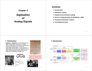
  • 1. Chapter 2 p Digitization Digitization of Analog Signals Contents Contents 1. Introduction 2. Waveform coding 3. Subband and transform coding g 4. Source coding (Analysis-by-Synthesis - AbS) 5 Vocoders (Parametric coders) 5. Vocoders (Parametric coders) 6. Concluding remarks 2 1. Introduction Digitizing or digitization: the representation of an object, image, sound, document or a (analog) signal by a discrete set of its points or samples that could receive limited values The result is could receive limited values. The result is called digital representation or, more specifically, a digital image, for the object, and digital form, for the signal. Strictly speaking, digitizing means simply f capturing an analog signal in digital form. T ê ô Độ lậ ủ Chí h hủ Tuyên ngôn Độc lập của Chính phủ Lâm thời nước Việt Nam Dân chủ Cộng hoà, ngày 2-9-1945. (Văn bản scan). Bảo tàng Lịch sử Quốc gia. Format 3 1. Introduction Digital info. E d Transmit Pulse d l t S l Q ti Format Textual info. Analog source Encode modulate Sample Quantize Channel Pulse waveforms Bit stream Format Analog info. Demodulate/ Detect Receive Low-pass filter Decode wave o s Format Textual Analog info. i k Textual info. Digital info. sink 4
  • 2. 1. Introduction  Speech coding is the process of obtaining a compact representation of voice signals for efficient transmission over band-limited wired and wireless channels d/ t Speech coding and/or storage.  Speech coders are lossy, i.e. the decoded signal is different from the original.  The goal in speech coding is to minimize the distortion at a given bit rate, or i i i th bit t t h i di t ti  Categories:  Waveform coding  Subband and transform coding minimize the bit rate to reach a given distortion. LPC-AS: Linear Prediction g  Source (analysis-by-synthesis) coding  Vocoders Characteristics of Standardized Speech Coding Algorithms in Each of Four Broad Categories LPC-AS: Linear Prediction Coding - Analysis-by-Synthesis Speech Coder Class Rates (kbps) Complexity Standardized Applications Waveform coders 16-64 Low Landline telephone Subband coders 12-256 Medium Teleconferencing, audio LPC AS 4 8 16 High Digital cellular LPC-AS 4.8-16 High Digital cellular LPC vocoder 2.0-4.8 High Satellite telephony, military 5 R t BW St d d St d d A Representative Sample of Speech Coding Standards Application Rate (kbps) BW (kHz) Standards Organization Standard Number Algorithm Year Landline telephone 64 16-40 16 40 3.4 3.4 3 4 ITU ITU ITU G.711 G.726 G 727 μ-law or A-law PCM ADPCM ADPCM 1988 1990 1990 16-40 3.4 ITU G.727 ADPCM 1990 Tele conferencing 48-64 16 7 3.4 ITU ITU G.722 G.728 Split-band ADPCM Low-delay CELP 1988 1992 Digital cellular 13 12 2 3.4 3 4 ETSI ETSI Full-rate EFR RPE-LTP ACELP 1992 1997 12.2 7.9 6.5 8.0 4 75 12 2 3.4 3.4 3.4 3.4 3 4 ETSI TIA ETSI ITU ETSI EFR IS-54 Half-rate G.729 AMR ACELP VSELP VSELP ACELP ACELP 1997 1990 1995 1996 1998 4.75-12.2 1-8 3.4 3.4 ETSI CDMA-TIA AMR IS-96 ACELP QCELP 1998 1993 Multimedia 5.3-6.3 2.0-18.2 3.4 3.4-7.5 ITU ISO G.723.1 MPEG-4 MPLPC, CELP HVXC, CELP 1996 1998 S t llit 4 15 3 4 INMARSAT M IMBE 1991 Satellite telephony 4.15 3.6 3.4 3.4 INMARSAT INMARSAT M Mini-M IMBE AMBE 1991 1995 Secure communi- ti 2.4 2.4 4 8 3.4 3.4 3 4 DDVPC DDVPC DDVPC FS1015 MELP FS1016 LPC-10e MELP CELP 1984 1996 1989 cations 4.8 16-32 3.4 3.4 DDVPC DDVPC FS1016 CVSD CELP CVSD 1989 1987 6 2 1 B i f Si l Di iti ti 2. WAVEFORM CODING 2.1. Basis of Signal Digitization 2.1.1.1 The sampling theorem 2.1.1 The Nyquist Sampling  Simply referred to of other names such as Shannon sampling theorem, Nyquist-Shannon-Kotelnikov, p g y Whittaker-Shannon-Kotelnikov, Whittaker-Nyquist-Kotelnikov- Shannon, WKS, etc., as well as the Cardinal Theorem of Interpolation Cardinal Theorem of Interpolation Theory.  To be a fundamental result in the field of information theory, in particular Hypothetical spectrum of a band-limited signal as a function of frequency y, p telecommunications and signal processing. “Exact reconstruction of a continuous-time baseband signal from its g samples is possible if the signal is band-limited and the sampling frequency is greater than twice the signal bandwidth.” 7 2.1.1.1 The sampling theorem …  The assumptions necessary to prove the theorem form a mathematical model that is only an idealized approximation of any real-world situation. The conclusion, that perfect reconstruction is possible, is mathematically correct for the model but only an approximation for actual signals and actual for the model, but only an approximation for actual signals and actual sampling techniques.  The signal x(t) is band-limited to a one-sided baseband bandwidth if: X(f ) 0 f ll | f | > B X(f ) = 0 for all | f | > B.  Then the sufficient condition for exact reconstructability from samples at a uniform sampling rate (in samples per unit time) f > 2B i l tl B < f /2 fs > 2B, or equivalently, B < fs/2.  2B is called the Nyquist rate and is a property of the bandlimited signal, while fs/2 is called the Nyquist frequency and is a property of this sampling system.  The time inter al bet een s ccessi e samples is referred to as the sampling  The time interval between successive samples is referred to as the sampling interval T ≡ 1/fs and the samples of x(t) are denoted by x[n] ≡ x(nT), n Î  (intergers).  Including two processes: sampling and reconstruction  Including two processes: sampling and reconstruction. 8
  • 3. 2.1.1.1 The sampling theorem …  Sampling process: The continuous signal varying over time is sampled by measuring the signal's value every T units of time (or space), which is called the sampling interval.  Reconstruction process of the original signal is an interpolation process that mathematically defines a continuous-time signal x(t) from the discrete samples x[n] and at times in between the sample instants nT by the following procedure: Each sample value is multiplied by the sinc function scaled so that the zero-crossings of the sinc function occur at the sampling instants and that the sinc function's central point is shifted to the time of that sample, nT. All of these shifted and scaled functions are then added together to recover the these shifted and scaled functions are then added together to recover the original signal. The scaled and time-shifted sinc functions are continuous making the sum of these also continuous, so the result of this operation is a continuous signal. This procedure is represented by the Whittaker-Shannon g p p y interpolation formula:         sin ( / ) sin ( / ) ( ) ( ) s s s s f t n f f t n f x t a a f x t dt               ( ) ( ) ( / ) ( / ) n n s n s s s s x t a a f x t dt f t n f f t n f         9 2.1.1.1 The sampling theorem … 10 2.1.1.1 The sampling theorem … Time domain Frequency domain ) ( ) ( ) ( t x t x t xs    ) ( ) ( ) ( f X f X f Xs    | ) ( | f X ) (t x | ) ( | f X ) (t x | ) ( | f Xs ) (t xs | ) ( | f s 11 2.1.1.2. Aliasing effect LP filter Nyquist rate aliasing  Original file (sampling frequency 44 1 kHz stereo) Demo!!!  Original file (sampling frequency 44.1 kHz, stereo)  Downsampling to 11.025 kHz without prefiltering (mono)  Downsampling to 11.025 kHz with prefiltering (mono) 12
  • 4. 2.1.1.2. Aliasing effect …  Examples of reconstruction problems due to aliasing p p g 13  I l li 2.1.1.3. How to sampling?  Impulse sampling  Natural sampling  Sample and hold 14 2.1.1.3. How to sampling? … Impulse sampling 15 2.1.1.3. How to sampling? … Natural sampling 16
  • 5. 2.1.1.3. How to sampling? … Sample and hold 17 2.1.1.4. Bandpass (under) sampling  B i id What are about the problems with  Basic idea the problems with sampling bandpass signals? 18  Resulting conditions needed for aliasing-free BP sampling Allowed (white) and forbidden (shaded) sampling frequencies 19  Example: Consider FM radio (in Vietnam) operating on the frequency band [fL ÷ fH] = [88 ÷ 108] MHz. The bandwidth W = fH - fL = 20 MHz. The sampling di i conditions: Therefore, k can be 1, 2, 3, 4, or 5. k = 5 gives the lowest sampling frequencies i t l 43 2 f 44 MH ( i f d li ) I thi th           1 5.4 = 108 MHz / 20 MHz k interval 43.2 < fs < 44 MHz (a scenario of undersampling). In this case, the signal spectrum fits between 2 and 2.5 times the sampling rate (higher than 86.4 ÷ 88 MHz but lower than 108 ÷ 110 MHz). Stringent antialias filtering!!! A lower value of k will also lead to a useful sampling rate For example A lower value of k will also lead to a useful sampling rate. For example, using k = 4, the FM band spectrum fits easily between 1.5 and 2.0 times the sampling rate, for a sampling rate near 56 MHz (multiples of the Nyquist frequency being 28, 56, 84, 112, etc.). Simpler antialias filtering!!! 20 2.1.1.5. Generalization: Under/critical/over sampling (Lấy mẫu dưới/tới/quá hạn) … may be overloaded!!!
  • 6. 2.1.2. Quantisation  A lit d ti i M i l f  Amplitude quantizing: Mapping samples of a continuous amplitude waveform to a finite set of amplitudes.  Uniform (linear) quantizing: Out ( ) q g In ed Quantize values 21 2.1.2. Quantisation …  Example: 111 3.1867 Amplitude x(t)  Example: ( T ) l d l quant. levels 111 3.1867 110 2.2762 101 1.3657 x(nTs): sampled values boundaries 100 0.4552 011 -0.4552 ( T ) ti d l boundaries 011 0.4552 010 -1.3657 001 -2.2762 Ts: sampling time xq(nTs): quantized values 00 . 76 000 -3.1867 t PCM codeword 110 110 111 110 100 010 011 100 100 011PCM sequence 22  Quantizing (roundoff) error: The difference between the input and output 2.1.2. Quantisation …  Quantizing (roundoff) error: The difference between the input and output of a quantizer:  Bernard Widrow showed that if the input random variable has a band- limited characteristic function then the input distribution can be recovered ) ( ) ( ˆ ) ( t x t x t e   limited characteristic function, then the input distribution can be recovered from the quantized-output distribution, and the quantization noise density is uniform. M d l f i i i P f i i i ) (t x ) ( ˆ t x Model of quantizing noise ) (x q y  Quantizer Process of quantizing noise ) ( ) ( ) (t e ) (t x ) ( ˆ t x AGC x ) ( q y ˆ ( ) ( ) ( ) e t x t x t   + x ( ) e t 23 ( ) 2.1.2. Quantisation …  Quantizing error types:  Granular or linear errors happen for inputs within the dynamic range of quantizer  Saturation errors happen for inputs outside the dynamic range of quantizer o Saturation errors are larger than linear errors o Saturation errors can be avoided by proper tuning of AGC  Quantization noise variance (linear):  Average quantization noise power 2 2 q    Signal peak power 12   2 2 2 p L q V  M l b d !!!  Signal power to average quantization noise power 4 p 2 2 3 p V S L       Matlab demo!!! 24 2 3 q L N       
  • 7. Statistical of speech amplitudes 1.0 nction 2.1.2. Quantisation … Statistical of speech amplitudes 0.5 ty density fun  For a fixed, uniform quantizer, an input signal with an amplitude 0.0 1.0 2.0 3 0 Probabilit less than full load will have a lower SQNR than a signal whose amplitude occupies the full dynamic range of the quantizer  Such a variation in performance (SQNR) as a function of quantizer input signal amplitude is particularly detrimental for speech, since low amplitude 1.0 3.0 Normalized magnitude of speech signal dynamic range of the quantizer (but without overload). g p p y p , p signals can be very important perceptually.  In speech, weak signals are more frequent than strong ones. Speech is generally stated to have a gamma or Laplacian probability density, which is hi hl k d b t highly peaked about zero.  Using equal step sizes (uniform quantizer) gives low SQNR for weak signals and high SQNR for strong signals.  Adjusting the step size of the quantizer by taking into account the speech  Adjusting the step size of the quantizer by taking into account the speech statistics improves the SNR for the input range. 25 2.1.2. Quantisation … Uniform vesus non-uniform quantization  Uniform (linear) quantizing:  No assumption about amplitude statistics and correlation properties of the No assumption about amplitude statistics and correlation properties of the input.  Not using the user-related specifications.  Robust to small changes in input statistic by not finely tuned to a specific set g p y y p of input parameters.  Simply implemented.  Application of linear quantizer: Signal processing, graphic and display applications, process control applications.  Non-uniform quantizing:  Using the input statistics to tune quantizer parameters.  Larger SNR than uniform quantizing with same number of levels.  Non-uniform intervals in the dynamic range with same quantization noise variance. A li ti f if ti C l d f h  Application of non-uniform quantizer: Commonly used for speech. 26 N if ti ti 2.1.2. Quantisation … Non-uniform quantization  It is done by uniformly quantizing the “compressed” signal.  At the receiver, an inverse compression characteristic, called “expansion” is l d t id i l di t ti employed to avoid signal distortion. Compression + expansion companding Compression expansion companding ) (x C y  x̂ ) (t y ) (t x ) ( ˆ t y ) ( ˆ t x ) ( y x x ŷ Compressing Quantizing Channel Expanding T itt R i Channel Transmitter Receiver 27 2.2. Pulse-Code Modulation - PCM  A digital representation of an analog signal where the magnitude of the signal is sampled regularly at uniform intervals, then quantized to a series of symbols in a digital (usually binary) code symbols in a digital (usually binary) code.  Has been used in digital telephone systems since 1940s and is also the standard form for digital audio in computers and the compact disc. p p  Laid the foundation for today’s digital transmission.  Applications: T/E-carrier, Audio CD, DVD, Blu-ray, pp y HDMI, WAV file, …  4-step processing:  Band-limited filtering S li Ralph Miller – former technical staff of Bell Labs in the 1940s 2 2 1 Band limited (antialias) filtering  Sampling  Quantizing  Coding in the 1940s. The inventor of PCM. 2.2.1. Band-limited (antialias) filtering  Voice signal is frequency constrained around 4 kHz by a lowpass filter. 28
  • 8. 2.2.2. Sampling (Time discretization)  fs = 8 Kilo-samples/sec or Ts = 125 μs. µ-law algorithm s p s μ 2.2.3. Quantisation (Amplitude discretization)  The µ-law algorithm: A companding algorithm, primarily used in the digital telecommunication systems of North America and Japan.  Algorithm types: Two forms - analog version, and quantized digital version.  Continuous: For a given input x, the equation for μ-law encoding is where μ = 255 (8 bits) in the North American and Japanese standards. μ-law expansion is then given by the inverse equation: μ p g y q  Discrete: Defined in ITU-T Recommendation G 711 Piece-wise linearly  Discrete: Defined in ITU-T Recommendation G.711. Piece-wise linearly approximated by 15 cords/segments. 29 A l l ith 2.2.3. Quantisation… A-law algorithm  Standard companding algorithm, used in European digital communications systems to optimize, i.e., modify, the dynamic range of an analog signal for digitizing digitizing.  Continuous: For a given input x, the equation for A-law encoding is as follows, where A is the compression parameter. In Europe, A = 87.7; the value where A is the compression parameter. In Europe, A 87.7; the value 87.6 is also used. A-law expansion is given by the inverse function,  Discrete: Defined in ITU T Recommendation G 711 Piece wise linearly  Discrete: Defined in ITU-T Recommendation G.711. Piece-wise linearly approximated by 13 cords/segments 30 2.2.3. Quantisation… 15-segment µ-law 13-segment A-law Discrete forms of non-uniform quantization 31 Quantized μ-law algorithm 14 bit binary linear input code 8 bit compressed code  μ-law 2.2.4. Coding 14 bit binary linear input code 8 bit compressed code +8159 to +4063 in 16 intervals of 256 1000ABCD +4062 to +2015 in 16 intervals of 128 1001ABCD +2014 to +991 in 16 intervals of 64 1010ABCD μ encoding thus takes a 14-bit signed linear audio sample +990 to +479 in 16 intervals of 32 1011ABCD +478 to +223 in 16 intervals of 16 1100ABCD +222 to +95 in 16 intervals of 8 1101ABCD audio sample as input and converts it to an 8 bit value +94 to +31 in 16 intervals of 4 1110ABCD +30 to +1 in 15 intervals of 2 1111ABCD 0 11111111 as follows: PXYZABCD  A bias of 33 is −1 01111111 −31 to −2 in 15 intervals of 2 0111ABCD −95 to −32 in 16 intervals of 4 0110ABCD  A bias of 33 is added to the absolute input value enabling th d i t −223 to −96 in 16 intervals of 8 0101ABCD −479 to −224 in 16 intervals of 16 0100ABCD −991 to −480 in 16 intervals of 32 0011ABCD 2015 t 992 i 16 i t l f 64 0010ABCD the endpoints of each chord to become powers of two, −2015 to −992 in 16 intervals of 64 0010ABCD −4063 to −2016 in 16 intervals of 128 0001ABCD −8159 to −4064 in 16 intervals of 256 0000ABCD p , also reducing max to 8159. 32
  • 9. Quantized A-law algorithm 2.2.4. Coding… Q g 13 bit binary linear input code 8 bit compressed code +4096 to +2048 in 16 intervals of 128 1111ABCD +2047 to +1024 in 16 intervals of 64 1110ABCD  A-law encoding thus takes a 13-bit +1023 to +512 in 16 intervals of 32 1101ABCD +511 to +256 in 16 intervals of 16 1100ABCD +255 to +128 in 16 intervals of 8 1011ABCD 13-bit signed linear audio sample as +127 to +64 in 16 intervals of 4 1010ABCD +63 to +32 in 16 intervals of 2 1001ABCD +31 to 0 in 16 intervals of 2 1000ABCD input and converts it to an 8 bit value as −31 to −1 in 16 intervals of 2 0000ABCD −63 to −32 in 16 intervals of 2 0001ABCD −127 to −64 in 16 intervals of 4 0010ABCD value as follows: −255 to −128 in 16 intervals of 8 0011ABCD −511 to −256 in 16 intervals of 16 0100ABCD −1023 to −512 in 16 intervals of 32 0101ABCD 2047 t 1024 i 16 i t l f 64 0110ABCD −2047 to −1024 in 16 intervals of 64 0110ABCD −4096 to −2048 in 16 intervals of 128 0111ABCD 33 Companding of μ-law and A-law algorithms 2.2.4. Coding… Companding of μ-law and A-law algorithms dBm0 - Power in dBm measured at a zero transmission level point dBFS - dB relative to full scale (ex: 50% of peak power → -3 dBFS) 34 2.2.4. Coding…  PCM signals is considered as a part of international connection.  Quantisation noise must guarantee the performance of existing analog routes.  As in referencing network, for 1 link (S/N)q ≥ 22 dB with the average dynamic range of voice from -25 to -5 dBm. The total referencing route includes 14 links, adding 10log14 = 11.46 dB on the budget. So, (S/N)qTotal = 33 46 dB 33.46 dB.  This needs a 7-bit coder. Providing other degradation requires 8-bit coder.  The code word: PXYZABCD.  Finally before transmission the entire codeword is inverted since low  Finally, before transmission, the entire codeword is inverted, since low amplitude signals tend to be more numerous than large amplitude signals. Consequently, inverting the bits increases the density of positive pulses on the transmission line, which improves the hardware performance. p p  The μ-law algorithm provides a slightly larger dynamic range than the A- law at the cost of worse proportional distortion for small signals.  By convention, A-law is used for an international connection if at least one y country uses it. 35 2.3. Differential Pulse-Code Modulation - DPCM m(t)  Basic idea: PCM tries to represent sample amplitudes → wasting “resource” when adjacent samples quite resemble one another t quite resemble one another. Encoding the differences between sample amplitudes is more efficient → DPCM  DPCM: A procedure of converting an analog into a digital signal in which an analog signal is sampled and then the difference between the actual sample value and its predicted value is quantized and then encoded forming a digital l P di t d l i b d i l l value. Predicted value is based on previous sample or samples.  Most source signals show significant correlation between successive samples so encoding using redundancy in sample values results in lower bit rate.  R li ti f thi b i t i b d t h i di ti t  Realization of this basic concept is based on a technique predicting current sample value based upon previous sample(s) and encoding the difference between actual value of sample and predicted value (prediction error).  A form of predictive coding DPCM compression depends on the prediction  A form of predictive coding. DPCM compression depends on the prediction technique, well-conducted prediction techniques → good compression rates. 36
  • 10.  Usually a linear predictor is used (linear predictive coding):  Delta Modulation: 1-bit predictor 37  A predictor can be realised with a tapped delay line to form a transversal filter.  Delay line: “hangs onto" (delays) past samples  Tapped: “tap into" line to pick up the desired signals  The an are the tap gains, calculated according to some “best fit" algorithm (e g minimum mean squared error) (e.g., minimum mean squared error) ( ) x n ( ) ( ) p x n 38  Small signal variation of variation of DPCM compared to PCM means l d d less coded bits needed.  Also, the signal signal statistics improved. 39  Signal distortions due to intraframe DPCM coding  Granular noise: random noise in flat areas of the picture, waveform Granular noise: random noise in flat areas of the picture, waveform  Edge busyness: jittery appearance of edges (for video)  Slope overload: blur of high-contrast edges, Moire patterns in periodic tructures. 40
  • 11. 41 2.4. Adaptive DPCM - ADPCM  Voice signal is not a strictly stationary but quasi-stationary process, namely, its variance and autocorrelation slowly varies by time.  Fixed stepsize uniform quantization might not result in quantization noise p q g q power of constant q2/12.  Adaptively change the quantizing step size to maintain quantization noise power constant (vector quantization method). Typically, the adaptation to signal statistics in ADPCM consists simply of an adaptive scale factor before quantizing the difference in the DPCM encoder.  Adaptively change the predictor (tap gains an) to reduce predictive signal distortions (vector prediction method) distortions (vector prediction method).  Resulting in coded bit rate of 16, 24, 32, 40 Kbps. 42 ITU-T ADPCM speech codec standard G.726 ADPCM encoder 43 G.726 ADPCM decoder 44
  • 12. 3. SUBBAND AND TRANSFORM CODING 3 1 P i i l 3.1. Principles  An analysis filterbank is first used to filter the signal into a number of frequency bands and then bits are allocated to each band by a certain criterion.  H b d tl f id b d di t hi h bit t h d  Has been used mostly for wideband medium to high bit rate speech coders and for audio coding.  For example, in G.722, ADPCM speech coding occurs within two subbands, and bit allocation is set to achieve 7 kHz audio coding at rates of 64 kbps or and bit allocation is set to achieve 7-kHz audio coding at rates of 64 kbps or less.  A speech production model is not used, ensuring is not used, ensuring robustness to speech in the presence of background noise, and to non-speech Hi h lit sources. High-quality compression can be achieved by incorporating masking properties of the g p p human auditory system. 45  Not widely used for speech coding today, but it is expected that new standards for wideband coding and rate-adaptive schemes will be based sta da ds o deba d cod g a d ate adapt e sc e es be based on subband coding or a hybrid technique that includes subband coding. This is because subband coders are more easily scalable in bit rate than standard CELP techniques, an issue which will become more critical for high quality speech and audio transmission over wireless communication high-quality speech and audio transmission over wireless communication channels and the Internet, allowing the system to seamlessly adapt to changes in both the transmission environment and network congestion. 3.2. Example: MPEG-1 Layer 3 (mp3) 46 4. SOURCE CODING 4.1. Speech Production Model  Speech is generated by pumping air from the lung through the g g vocal tract consisting of throat, nose, mouth, palate, tongue, teeth and lips. Lax vocal Nasal cavity Velum Nasal sound output cords - Open for breathing Vocal Folds/ Cords Pharyngeal cavity Tongue Oral cavity output Oral Lungs Trachea hump sound output T d l Lungs Tensed vocal cords - Ready to vibrate 47  Voiced sounds: The 4.2. Voice/Voiceless Sounds  Voiced sounds: The tense vocal chords are vibrating and the airflow gets modulated. The oscillation frequency of the vocal chords is called 'pitch'. The vocal tract colours the spectrum of voiced voiceless colours the spectrum of the pulsating air flow in a sound-typical manner.  Voiceless sounds: The vocal chords are loose and white-noise-like turbulences are formed at bottlenecks in the vocal bottlenecks in the vocal tract. The remaining vocal tract colours the turbulating airflow more or less depending on the position of the bottleneck. Demo! 48
  • 13. 4.3. Formants  One major property of speech is its correlation, i.e. successive samples of a speech signal are similar Vowel /a/ in short term speech signal are similar.  The short-term correlation of successive speech samples has consequences for the short-term spectral envelopes (< 10 ms).  These spectral envelopes have a few local maxima, the so called 'formants' which correspond to resonance frequencies of the human vocal tract. Speech consists of a succession of sounds, the so-called phonemes. While speaking, humans continuously change the setting of their vocal tract in order to produce different resonance frequencies (formants) and therefore different sounds different resonance frequencies (formants) and therefore different sounds.  This (short-term) correlation can be used to estimate the current speech sample from past samples. This estimation is called 'prediction'. Because the prediction is done by a linear combination of (past) speech samples, it is called 'linear prediction'. The difference between the original and the estimated signal is called 'prediction error signal'. 49 Vowel /a/: Spectral estimations of original estimations of original signal (green), predicted signal with 10-th order short-term predictor (red) and frequency response of a 10-th order speech model filter based on the predictor coefficients predictor coefficients (blue). Four formants can easily be identified.  Ideally, all correlation is removed, i.e. the error signal is white noise. Only the error signal is conveyed to the receiver: It has less redundancy, therefore each bit carries more information. In other words: With less bits, we can transport the same amount of information i e have the same speech quality transport the same amount of information, i.e. have the same speech quality.  The calculation of the prediction error signal corresponds to a linear filtering of the original speech signal: The speech signal is the filter input, and the error signal is the output. Main component of this filter is the (short-term) predictor. signal is the output. Main component of this filter is the (short term) predictor. The goal of the filter is to 'whiten' the speech signal, i.e. to filter out the formants. That is why this filter is also called an 'inverse formant filter'. 50  While speaking, the formants continuously change → the short- term correlation also changes and the predictor must be adapted to the these changes. Thus, the predictor and the prediction error filter are LPC Filter and the prediction error filter are adaptive filters whose parameters must be continuously estimated from the speech signal. 4.4. Pitch  Voiced sounds as e.g. vowels have a periodic structure, i.e. their signal form repeats itself after some milliseconds the so-called pitch period T Its repeats itself after some milliseconds, the so called pitch period Tp. Its reciprocal value fp = 1/Tp is called pitch frequency. So there is also correlation between distant samples in voiced sounds.  This long-term correlation is exploited for bit-rate reduction with a so-called g p long-term predictor (also called pitch predictor).  Also the pitch frequency is no constant. Female speakers have higher pitch than male speakers. The pitch frequency varies in a speaker-typical manner. V i l d t d t h i di t t t ll d Voice-less sounds as consonants do not have a periodic structure at all, and mixed sounds with voice-less and voiced components also exist. 51  Thus, also the pitch predictor must be implemented as an adaptive filter, and the pitch period and the pitch gain must be continuously estimated from the speech signal. Vowel /a/ in long term 52
  • 14. 4.5. Spectrogram 0.3 “ee” “ee” “oh” “oh”  A useful representation of the speech signal, showing the signal's power distribution with respect to 0 0.1 0.2 plitude ee ee oh oh time and frequency.  The idea is to calculate the (short- term) power spectral densities (this i th d f -0.2 -0.1 Amp gives the power and frequency information) of successive (this gives the time information) fragments of the signal. 3500 4000 0 5 10 15 20 -0.3 g  Usually, the time is printed on the x- scale of a spectrogram and the frequency on the y-scale. The power 2000 2500 3000 ency (Hz) is coded in the color, for example red means high power and blue low power. 500 1000 1500 Freque 53 0 5 10 15 20 Time 4.6. Adaptive Predictive Coding  Only the parameters of the inverse formant filter and the inverse pitch filter  Only the parameters of the inverse formant filter and the inverse pitch filter plus the error signal are transmitted to the receiver. The receiver constructs the inverse filters, i.e. a pitch filter and a formant filter, and reconstructs the speech signal by inverse filtering of the error signal. This coding structure is known as ‘Adaptive Predictive Coding’ - APC.  APC is the basis for a variety of so-called waveform speech codecs which try to preserve the waveform of the speech signal. The idea is not to convey the p p g y error signal completely: Only an equivalent version is transferred, or a version carrying the main information. Thus we are saving bits. 54 4.7. RELP, MPE & RPE  B b d R id l E it d Li P di ti (BB RELP) O l l  Baseband Residual Excited Linear Prediction (BB-RELP): Only a low pass-filtered version of the error signal (also called residual) is conveyed to the receiver. The low pass-filtered version of the error signal can be down sampled and fewer samples have to be transmitted. The decoder must p p somehow regenerate the missing spectral components, this is done by simply repeating the spectral baseband information in the spectral domain (a number of zeros = down sampling factor are padded in the time domain between each sample) between each sample).  Multi-Pulse Excited Linear Prediction (MPE-LPC): The residual is substituted by a small number of impulses (all other samples are set to zero). Typically, 40 samples are replaced by 4 to 6 samples whose positions zero). Typically, 40 samples are replaced by 4 to 6 samples whose positions and values are determined one after the other by minimizing the mean square error (MSE) between the original and the synthesized speech signal.  Regular-Pulse Excited Linear Prediction (RPE-LPC): This is similar to MPE, but the pulses have a fixed distance. Only the position of the first pulse must be transferred to the receiver. The pulse amplitudes can be found by solving a linear equations. The GSM Full-Rate Codec is a mixture of an RPE and a BB-RELP codec: The down sampling factor is three and the down and a BB RELP codec: The down sampling factor is three, and the down sampled excitation signal with the highest energy is chosen. 55 4.8. CELP – Codebook Excited Linear Prediction  Modern algorithms (used in GSM, UMTS, LTE) have a limited storage of potential prediction error signals (the stochastic codebook), and the index of the best-fitting signal is transferred to the receiver → few bis transmitted.  In the coder, each prediction error signal is already vocal-tract filtered and the th th i d h i l i d t th i i l h i l b thus synthesized speech signal is compared to the original speech signal by applying an error measure, e.g. the MSE → 'analysis-by-synthesis'. Thus, a vector quantization of the original speech segment is performed.  The decoder has the same codebook available and can retrieve the best-  The decoder has the same codebook available and can retrieve the best fitting error signal with the index. CELP P i i l CELP Principle: Analysis-by- Synthesis. The best codebook vector is codebook vector is determined and afterwards the corresponding best i l i gain value is calculated. 56
  • 15.  This scheme results in low bit rates but the speech quality is inferior: Although intelligible, the codec sounds artificial and lacks naturalness because voiced (periodic) speech frames are no good reproduced.  Improvement can be done by performing an APC-like pitch analysis first. The calculated LTP delay and LTP gain values are used for inducing a pitch t t i t th t h ti d b k t i t th l i b structure into the stochastic codebook vectors prior to the analysis-by- synthesis. This idea is realized in the below scheme. 4.8.1. Open-Loop CELP Open-Loop CELP Principle: Analysis-by-Synthesis. The decoder is fully included in the coder Main part of the structure coder. Main part of the structure resembles an APC decoder. 57 4.8.2. Closed-Loop CELP  The LTP analysis can also be included into the Analysis-by-Synthesis resulting y y y y g in an even better reproduction of voiced frames, especially for small LTP delay values which are typical for female speakers → ‘Closed-loop’ CELP.  This is the basis for state-of-the-art speech codecs as ITU-T G.729, ETSI GSM Enhanced Fullrate Codec (EFR) etc works! Enhanced Fullrate Codec (EFR) etc. works! Closed-Loop CELP Principle: CELP Principle: LTP included in Analysis-by- Synthesis. 58 4.8.3. Improving CELP's Speech Quality The CELP codecs described here so far still do not sound good enough. Many g g y ideas resulted in a considerable improvement of the speech quality:  The stochastic codebooks were trained with real speech material (instead of simply white Gaussian noise).  More complex error measures were introduced: Very typical is an error weighting filter which is applied to the error signal before calculating the MSE: Thus, the perceptual error is minimized according to psychoacoustic results. f  Another idea is to use more than one stochastic codebook in order to further minimize the remaining error.  'Fractional' delays can improve the pitch regeneration. An oversampling filter is used to calculate intermediate samples of the past excitation signal of the is used to calculate intermediate samples of the past excitation signal of the vocal-tract filter, and the delay value is thus no more restricted to a multiple of the sampling period.  Better quantization techniques for the parameter values use the available bit  Better quantization techniques for the parameter values use the available bit rate more efficiently. Vector quantization of LPC coefficients or pitch parameters is often found. Also, other representations for the LPC coefficients improve their coding: E.g. Line Spectral Frequencies allow a representation of 10 LPC ffi i t ith l 28 bit 10 LPC coefficients with only 28 bits.  Post-filters in the decoder can slightly improve the perceived speech quality. 59  The analysis-by-synthesis is computationally very expensive → reduce the 4.8.4. CELP Implementation Considerations e a a ys s by sy t es s s co putat o a y e y e pe s e educe t e complexity (in terms of MIPs and MFLOPs). Most of the ideas concern the stochastic codebook: By using special structures, the computational cost of the vocal-tract filtering can be greatly simplified:  Unity Magnitude Codebook: The optimal stochastic excitation signal can also be searched in the frequency domain. If the Discrete Fourier Transforms of the codebook vectors all have the same magnitude and differ only in phase, the minimization procedure is greatly simplified minimization procedure is greatly simplified.  Vector-Sum CELP Codecs (VSELP) as e.g. the North American IS-54 have only a few base vector, and all other stochastic vectors are derived by a linear combination of these base vectors. Because the vocal-tract filter is a linear, only y the base vectors must be actually filtered, and the filtered stochastic vectors are calculated by a linear combination of the filtered base vectors.  Algebraic (structured) CELP Codecs (ACELP) as ITU-T G.729 and EFR use d b k E h t h l f l ≠ 0 d th l a sparse codebook: Each vector has only a few samples ≠ 0, and these samples only have values of -1 and +1 (resolving memory shortage & complexity problems). The properties of the codebook vectors can be optimized for the current speech segment by applying a signal-adaptive filtering. The search for p g y pp y g g p g the optimal excitation can be efficiently performed in the excitation domain after inverse vocal-tract filtering of the original speech signal. 60
  • 16. The most popular codebook structure is the interleaved pulse permutation code, in which, codevector consists of a set of interleaved permutation codes containing only few non-zero elements: pi = i + jd, j = 0, 1,…, 2M − 1, where pi is the pulse position, i is the pulse number, and d is the interleaving depth. The integer M is the number of bits describing the pulse positions. Example, interleaving depth d = 5, max number of pulses/tracks = 5, number of bits to represent the pulse positions M = 3 → p = i + j5 where i = 0 1 2 3 4 Track(i) Pulse positions (pi) 0 p0: 0, 5, 10, 15, 20, 25, 30, 35 1 p1: 1, 6, 11, 16, 21, 26, 31, 36 2 p2: 2, 7, 12, 17, 22, 27, 32, 37 M = 3 → pi = i + j5, where i = 0,1,2,3,4 and j = 0,1,2,…,7. For a given value of i, the set {pi} is known as ‘track,’ and the value of j defines 2 p2: 2, 7, 12, 17, 22, 27, 32, 37 3 p3: 3, 8, 13, 18, 23, 28, 33, 38 4 p4: 4, 9, 14, 19, 24, 29, 34, 39 g {pi} j the pulse position. From the codebook structure shown in the above table, the codevector, x(n), is given by, 4 ( ) ( - ), 0,1,...,39, i i x n n p n      where δ(n) is the unit impulse, αi are the pulse amplitudes (±1) and pi are the pulse positions. In particular, the codebook vector, x(n), is computed by placing the 5 unit pulses at the determined locations p multiplied with their signs (±1) 0 ( ) ( ), , ,..., 9, i i i p     the 5 unit pulses at the determined locations, pi, multiplied with their signs (±1) . The pulse position indices and the signs are encoded and transmitted. Note that the algebraic codebooks do not require any storage! 61 ACELP map 62 4.9. Adaptive Multi-Rate Codec - AMR  3G & 4G utilize the AMR codec. AMR offers several bitrates and can thus be adapted to the current channel conditions. AMR is nothing special, it is just an ACELP codec as described above. Different parameter settings lead to different speech qualities and bitrates different speech qualities and bitrates.  ETSI adopted ACELP for GSM telephony operating at multiple rates: 12.2, 10.2, 7.95, 6.7, 5.9, 5.15, and 5.75 kb/s. The bit rate is adjusted according to the traffic conditions. the traffic conditions.  The Adaptive Multi-Rate WideBand (AMR-WB) is an ITU-T wideband standard that has been jointly standardized with 3GPP, and it operates at rates 23.85, 23.05, 19.85, 18.25, 15.85, 14.25, 12.65, 8.85 and 6.6 kbps. The higher rates provide better quality where background noise is stronger.  The other two important speech coding standards are the Variable Rate Multimode WideBand (VMR-WB, adopted by 3GPP2) with the source coding t lli th bit t f ti ( t f 1 1/2 1/4 1/8 di t controlling the bit rates of operation (rates of 1,1/2,1/4,1/8 corresponding to 13.3, 6.2, 2.7 and 1 kbps) and the extended AMR-WB (AMR-WB+) addressing mixed speech and audio content, delivering high quality audio even at low bit rates. 63 Reflection coefficients coded as 4.10. GSM coder Short term LPC analysis (1) ( ) coefficients coded as Log. - Area Ratios (36 bits/20 ms) RPE parameters Input Pre- processing signal Short term analysis filter + RPE grid selection and coding (1) (2) (3) - p (47 bits/5 ms) (13 pulses) Long term analysis filter + RPE grid decoding and positioning (4) (5) 13 Kbps RPE-LTP coder (GSM 06.10 version LTP analysis LTP parameters (9 bits/5 ms) ( 8.1.1 Release 1999) To radio subsystem (1) Short term residual (2) Long term residual (40 samples) (3) Short term residual estimate (40 samples) (4) Reconstructed short term residual (40 samples) (5) Quantized long term residual (40 samples) subsystem ( ) g ( p ) Simplified block diagram of the RPE – LTP encoder 64
  • 17. 13 Kbps RPE-LTP coder (GSM 06.10 version 8.1.1 Release 1999) 4.10. GSM coder Reflection coefficients coded as Log. - Area Ratios (36 bits/20 ms) RPE grid decoding and positioning + Short term synthesis filter Post- processing Output signal positioning RPE parameters (47 bits/5 ms) filter Long term synthesis filter g signal (13 pulses) LTP parameters (9 bits/5 ms) From radio Simplified block diagram of the RPE - LTP decoder subsystem 65 4.11. Extended Adaptive Multi-Rate - Wideband (AMR-WB+) codec 3GPP TS 26.290 V11.0.0 (2012-09) HF signals folded in 0-Fs/4 kHz band HF encoding HF parameters Input signal L LHF RHF HF parameters preprocesing Input signal R Mono LF parameters HF encoding MLF RHF mode MHF Input signal HF parameters preprocesing and analysis filterbank ACELP/TCX encoding LF parameters MUX MLF Stereo parameters LLF MLF g M Down Mixing (L,R) to (M,S) Stereo encoding parameters RLF SLF Mono operation LF signals folded in 0-Fs/4 kHz band AMR-WB+ - Extended Adaptive Multi-Rate Wideband ACELP - Algebraic Code Excited Linear Prediction High-level structure of AMR-WB+ encoder g TCX - Transform coded excitation (transform-based core-coder) 66 4.11. Extended Adaptive Multi-Rate - Wideband (AMR-WB+) codec 3GPP TS 26.290 V11.0.0 (2012-09) HF parameters HF decoding LHF LHF HF parameters HF signals folded in 0-Fs/4 kHz band RHF HF decoding mode RHF MHF Output signal L synthesis filterbank and postprocesing Mono LF parameters DEMUX ACELP/TCX decoding MLF MHF Output signal R Output signal M Stereo parameters Stereo d di LLF RLF decoding RLF Mono operation AMR-WB+ - Extended Adaptive Multi-Rate Wideband ACELP - Algebraic Code Excited Linear Prediction TCX T f d d it ti (t f b d d ) High-level structure of AMR-WB+ decoder TCX - Transform coded excitation (transform-based core-coder) 67 5. LPC Vocoders  In practice all sounds have a mixed excitation which means that the excitation  In practice, all sounds have a mixed excitation, which means that the excitation consists of voiced and unvoiced portions. Of course, the relation of these portions varies strongly with the sound being generated.  An (over) simplification can be made in the sound production model by 'hard' ( ) p p y switch between voiced and unvoiced excitation. Thus the excitation signal is not transmitted at all but only some parameters describing it, e.g. its power. Such an algorithm produces really artificial speech and is known as a 'Vocoder' (Voice Coder) (Voice Coder). 68
  • 18.  This codec contains a simple classifier which decides whether the current frame is a silence, voiceless or voiced frame: The signal level determines if it is a silence frame or not, and if it is non-silence, the average zero-crossing rate determines if it is voiceless or voiced (in voiceless frames, there are more zero-crossings) more zero crossings).  The classifier result is feeded into a state-machine which takes the final decision whether the frame shall be treated as silence, voiced or voiceless (the idea is to smooth out changes from voiced/voiceless to silence). ( g )  Mixed voiced/voiceless excitations are not supported by this implementation.  In voiceless frames, only the mean signal amplitude and the predictor coefficients are calculated and conveyed to the decoder. y  In voiced frames, also the pitch lag is estimated (with a very simple block autocorrelation approach) and conveyed.  The decoder creates an excitation signal from the silence (just zeroes), g (j ) voiceless (just random noise) and voiced (just 1-pulses in a distance corresponding to the current estimated pitch lag) information and filters it with the adaptive vocal tract filter constructed with the transmitted LPC predictor coefficients predictor coefficients. 69 6. Concluding remarks Speech Coding Standards  Toll quality speech coder (digital wireline phone) - G.711 (A-LAW and μ-LAW at 64 kbits/sec) - G.721 (ADPCM at 32 kbits/ sec) - G.723 (ADPCM at 40, 24 kbps) - G.726 (ADPCM at 16,24,32,40 kbps)  Low bit rate speech coder (cellular phone/IP phone)  Low bit rate speech coder (cellular phone/IP phone) - G.728 low delay (16 Kbps, delay <2ms, same or better quality than G.721) - G. 723.1 (CELP Based, 5.3 and 6.4 kbits/sec) - G.729 (CELP based, 8 kbps) GS ( / / GS ) - GSM 06.10 (13/6.5 kbits/sec, simple to implement, used in GSM phones) Figure of Merit - Objective measure of distortion is SNR (Signal to noise ratio) j ( g ) - SNR does not correlate well with perceived speech quality Speech quality is often measured by MOS (mean opinion score) - 5: excellent - 4: good - 3: fair - 2: poor - 1: bad  PCM at 64 kbps with μ‐law or A‐law has MOS = 4.5 to 5.0 70 Speech Quality Versus Bit Rate For Common Classes of Codecs PCM 64Kbps noiseless PCM 64Kbps noise PCM 64Kbps noise GSM RPE-LPT 13Kbps QCELP-IS96a 7.5Kbps p CELP 4.8Kbps LPC 2.4Kbps 71 Thank you for your attention 72