Downloaded 16 times


![Self-Similarity Matrix
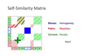
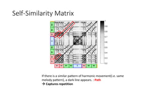
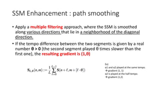
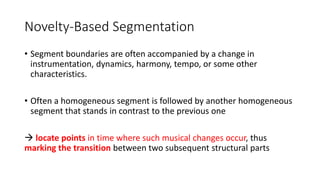
• SSM is doing a similar thing, but with itself this time.
Score of the cell (x, y) : similarity measure s(x, y)
(absolute value of the inner product)
N-square self-similarity matrix S ∈ RN×N
Where xn,xm ∈F (feature space), n,m∈[1:N]](https://image.slidesharecdn.com/mpch5-170403153553/85/Fundamentals-of-music-processing-chapter-5-14-320.jpg)
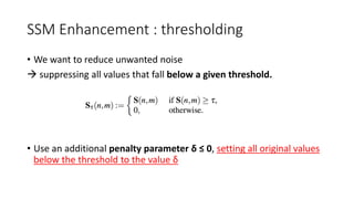
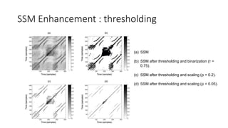
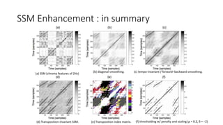
![SSM Enhancement : thresholding
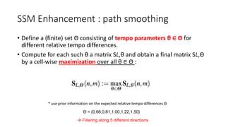
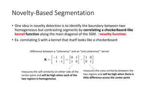
• Scaling from the range [τ,μ] [0,1]
( for μ := maxn,m{S(n,m)} > τ, otherwise all entries are set to zero)
• Choose τ in a relative fashion (ρ · 100%)
: keeping ρ · 100% of the cells with the highest values using a relative
threshold parameter ρ ∈ [0,1]
(Local strategy of setting τ in a column- and rowwise fashion)](https://image.slidesharecdn.com/mpch5-170403153553/85/Fundamentals-of-music-processing-chapter-5-34-320.jpg)
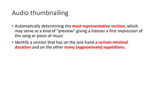

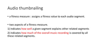
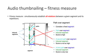

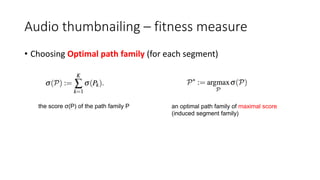

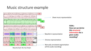
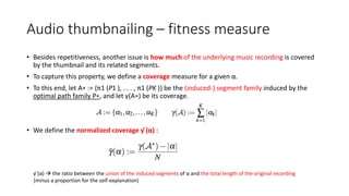
![Audio thumbnailing – fitness measure
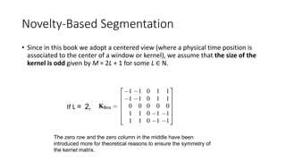
computing an optimal path family over a given segment α = [s : t] ⊆ [1 : N]
1) N × M submatrix Sα (segment α = [s : t] with M := |α|)
columns s : t of the self-similarity matrix S.
2) An accumulated score matrix D ∈ RN,M+1 by a recursive procedure.
(D : [1 : N] rows, [0 : M] columns)
3) Φ (n, m) : a set of predecessors of cell (n, m)
all cells that may precede (n,m) in a valid path family.
4) Accumulated score matrix :
5) Constraint conditions
: values of D for the remaining index pairs (n, m) with n = 1 or m ∈ {0, 1}
for n∈[2:N]
Complexity: O(MN)](https://image.slidesharecdn.com/mpch5-170403153553/85/Fundamentals-of-music-processing-chapter-5-46-320.jpg)
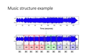
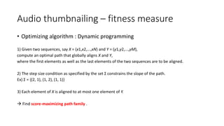
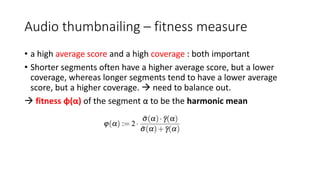
![Audio thumbnailing – fitness measure
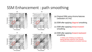
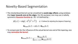
computing an optimal path family over a given segment α = [s : t] ⊆ [1 : N]
Submatrix Sα w/ α = [50 : 100]
Accumulated score matrix D
Optimal path family](https://image.slidesharecdn.com/mpch5-170403153553/85/Fundamentals-of-music-processing-chapter-5-47-320.jpg)
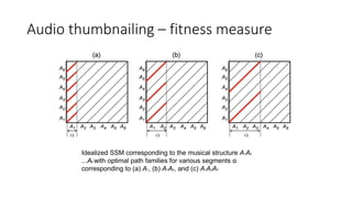

![Audio thumbnailing – scape plotting
• There are (N + 1)N /2 different segments α = [s : t] ⊆ [1 : N] where s,t ∈ [1 : N]
• Instead of considering start and end points, each segment can also be uniquely described by its center :
scape plot ∆ :](https://image.slidesharecdn.com/mpch5-170403153553/85/Fundamentals-of-music-processing-chapter-5-53-320.jpg)
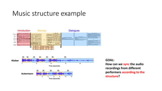
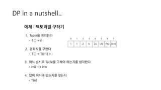
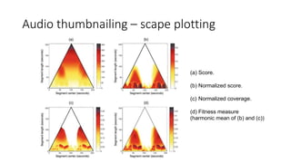
![Audio thumbnailing – scape plotting
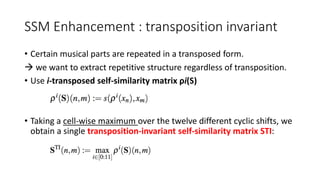
(b) α = α∗ = [68 : 89]
(corresponding to B2)
(c) α = [41 : 67]
(corresponding to B1
)
(d) α = [131 : 150]
(corresponding to A3 )
(e) α = [21 : 89]
(corresponding to A1B1B2)
the thumbnail segments of maximal fitness
(Choose maximum point)
c(α) = 78.5
|α| = 22](https://image.slidesharecdn.com/mpch5-170403153553/85/Fundamentals-of-music-processing-chapter-5-54-320.jpg)
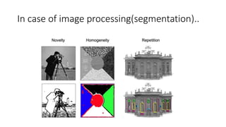
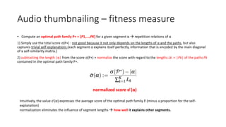
![Audio thumbnailing – scape plotting
α = α∗ = [68 : 89]
(corresponding to
B2)
α = [41 : 67]
(corresponding to B1 )
Recall that the introduced fitness measure slightly favors shorter segments
recording the B2-part is played faster than the B1-part, the fitness measure favors the B2-part
segment over the B1-part segment.
vs](https://image.slidesharecdn.com/mpch5-170403153553/85/Fundamentals-of-music-processing-chapter-5-55-320.jpg)
![Audio thumbnailing – scape plotting
Beatles song “Twist and Shout.”
The song contains a short harmonic phrase, a so-
called riff, which is repeated over and over again.
α∗ = [127 : 130] is very short and leads to a large
number of spurious induced segments.](https://image.slidesharecdn.com/mpch5-170403153553/85/Fundamentals-of-music-processing-chapter-5-57-320.jpg)

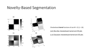
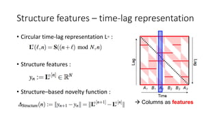
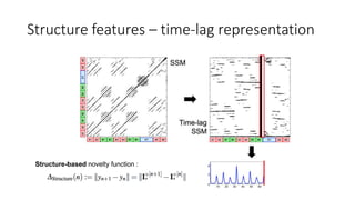
![Structure features – time-lag representation
• time-lag representation of S :
(for n∈[0:N−1] and l∈[−n:N−1−n])
Lines that are parallel to the main diagonal in S
become horizontal lines in L.](https://image.slidesharecdn.com/mpch5-170403153553/85/Fundamentals-of-music-processing-chapter-5-66-320.jpg)

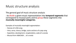
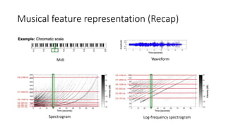
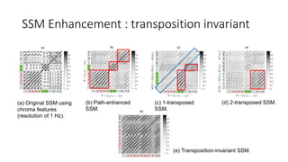
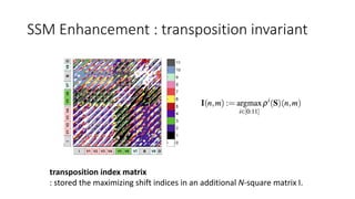
This document summarizes key aspects of chord recognition and music structure analysis from the book "Fundamentals of Music Processing". It discusses template-based and HMM-based chord recognition methods. For music structure analysis, it describes how a self-similarity matrix can be used to identify repetitive patterns in a song that correspond to musical parts or forms. Techniques are presented for enhancing the self-similarity matrix such as path smoothing, transposition invariance, and thresholding. Audio thumbnailing is introduced as a way to automatically select a representative section of a song using a fitness measure that balances repetitiveness and coverage of the song.