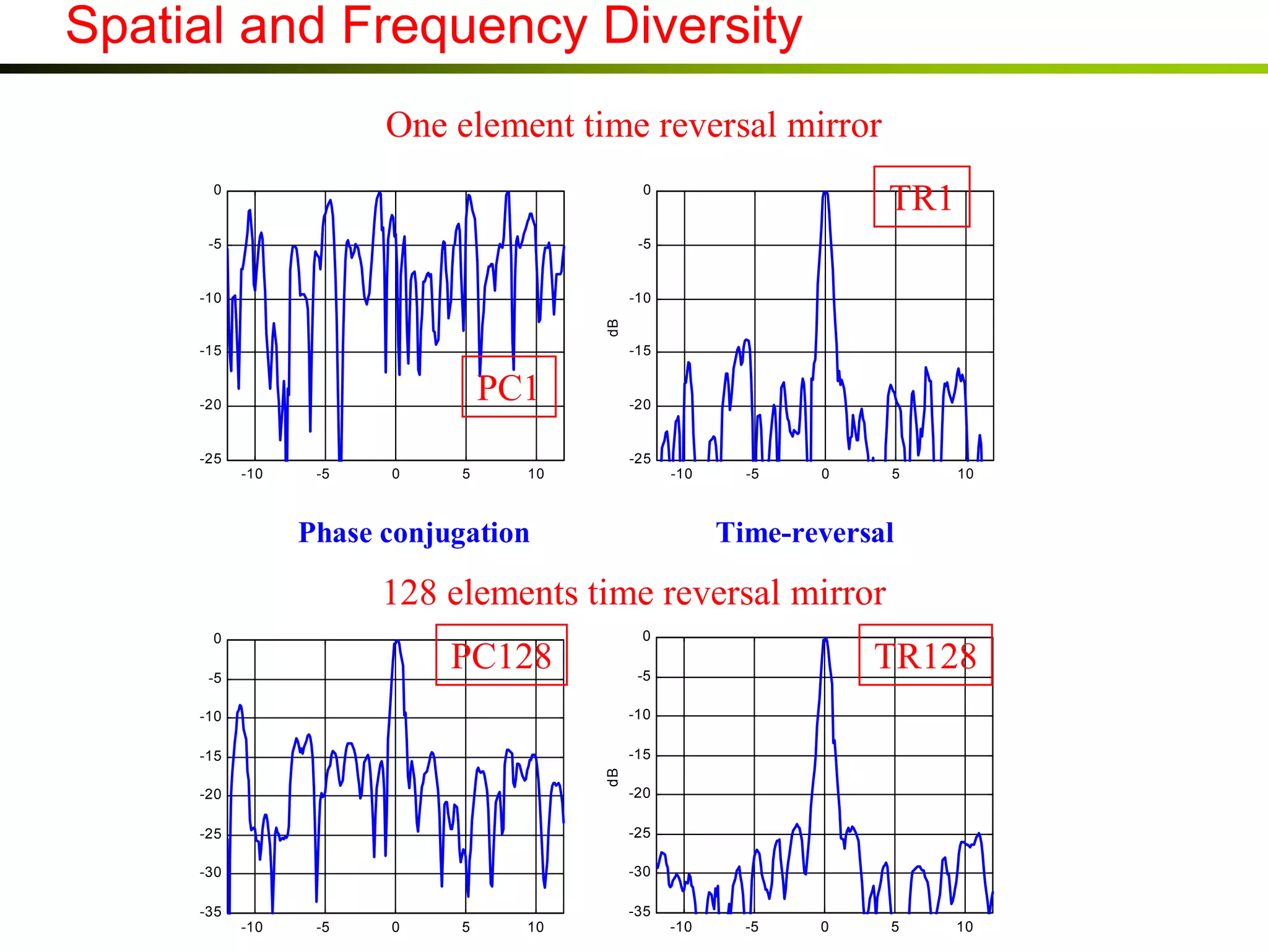
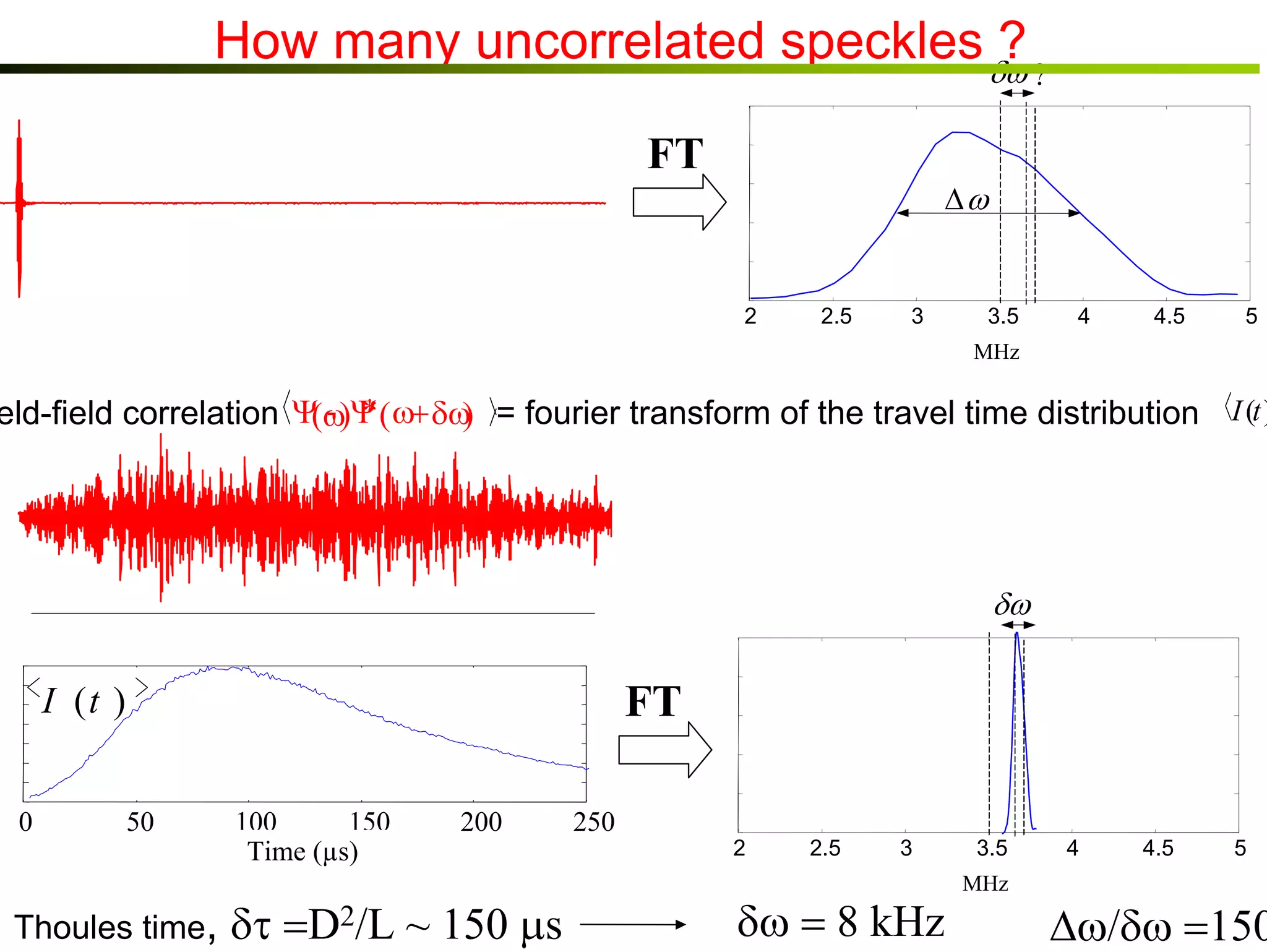
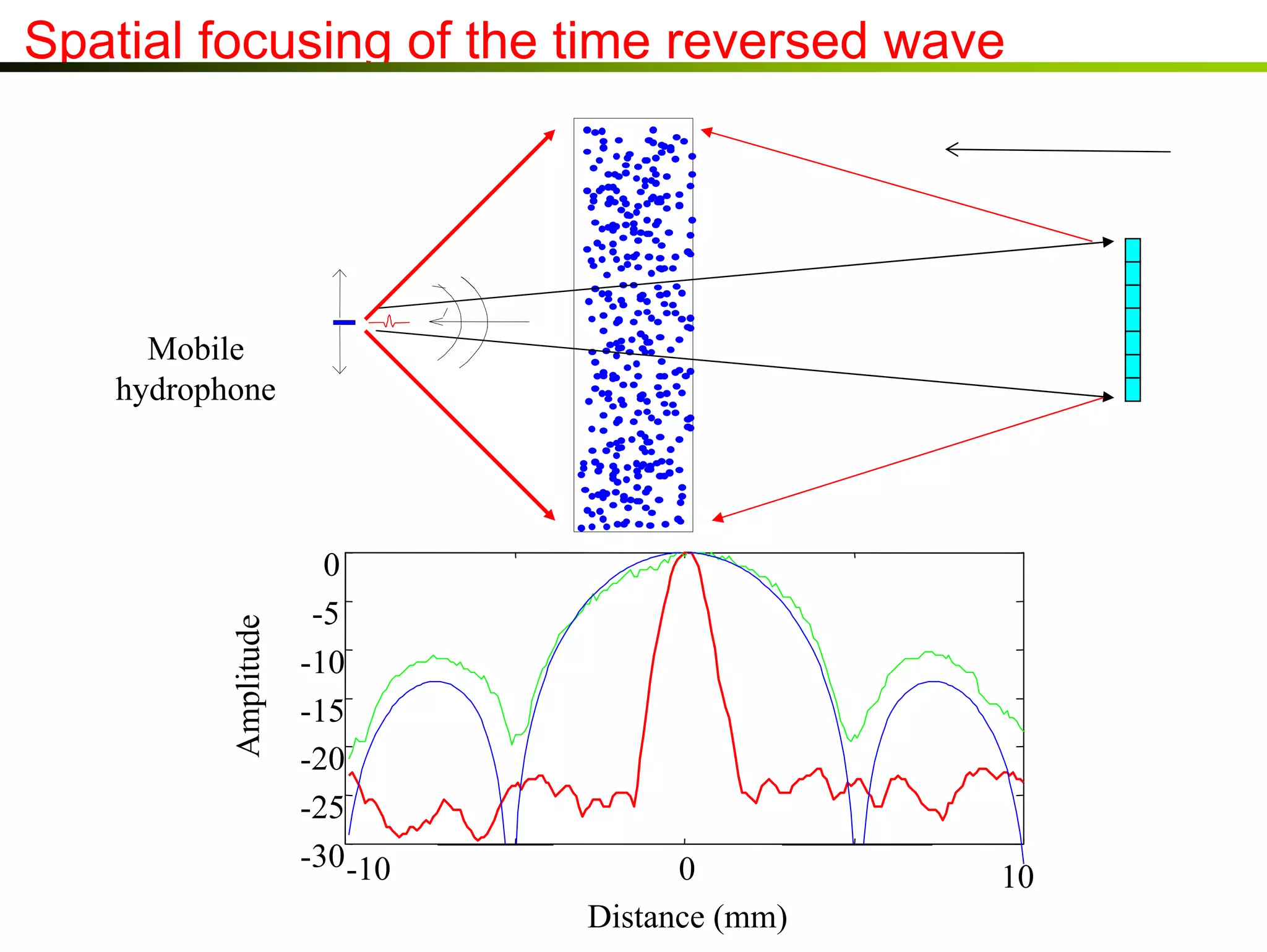
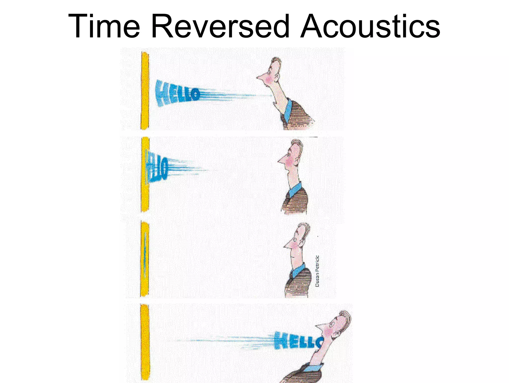
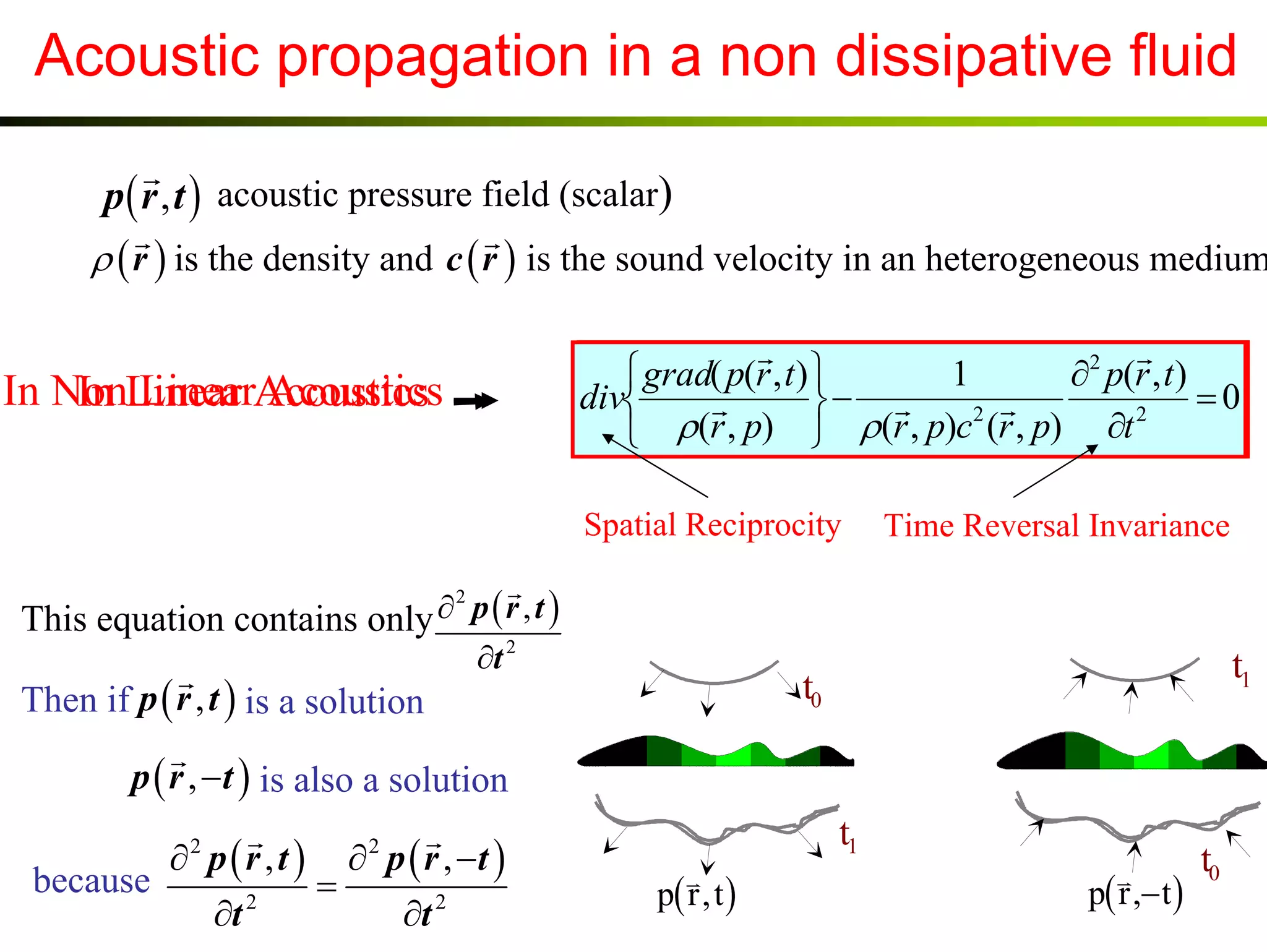
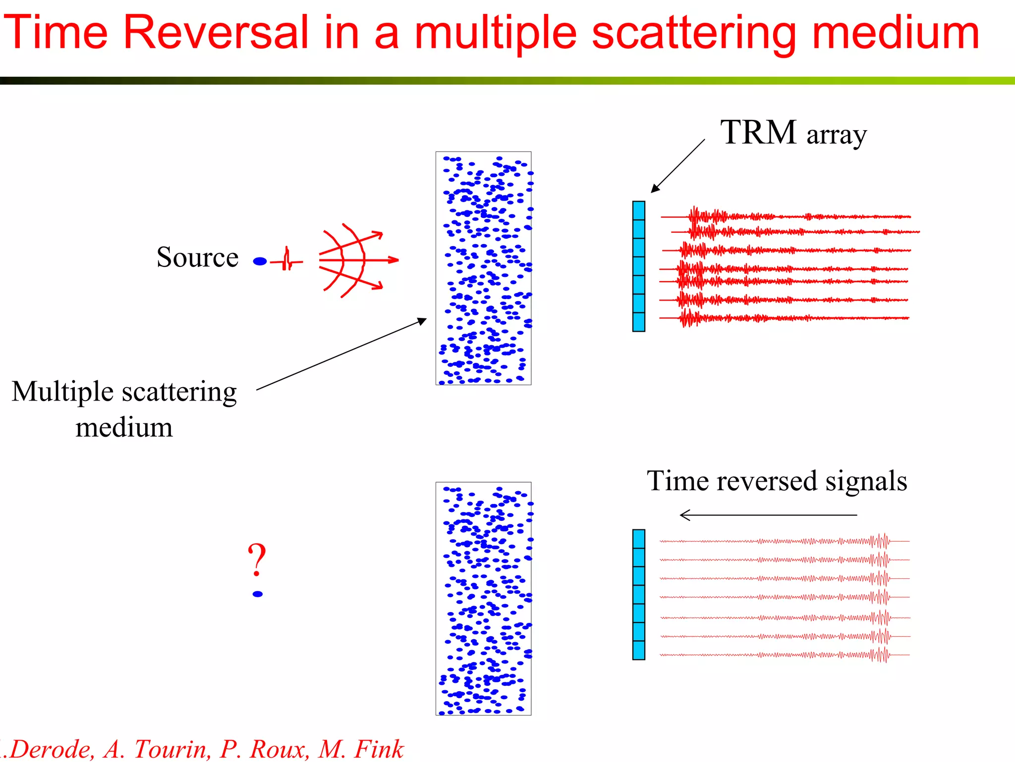
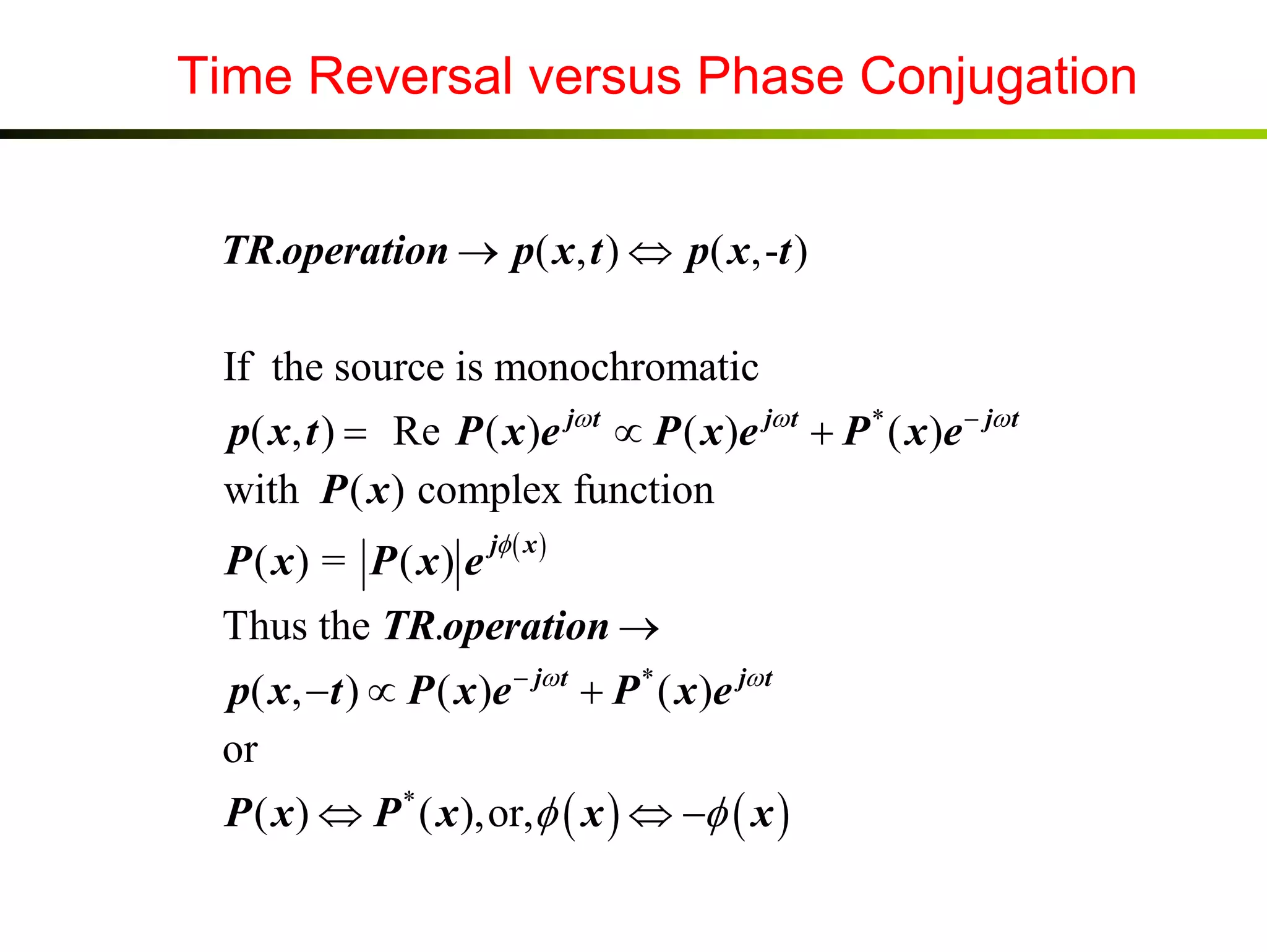
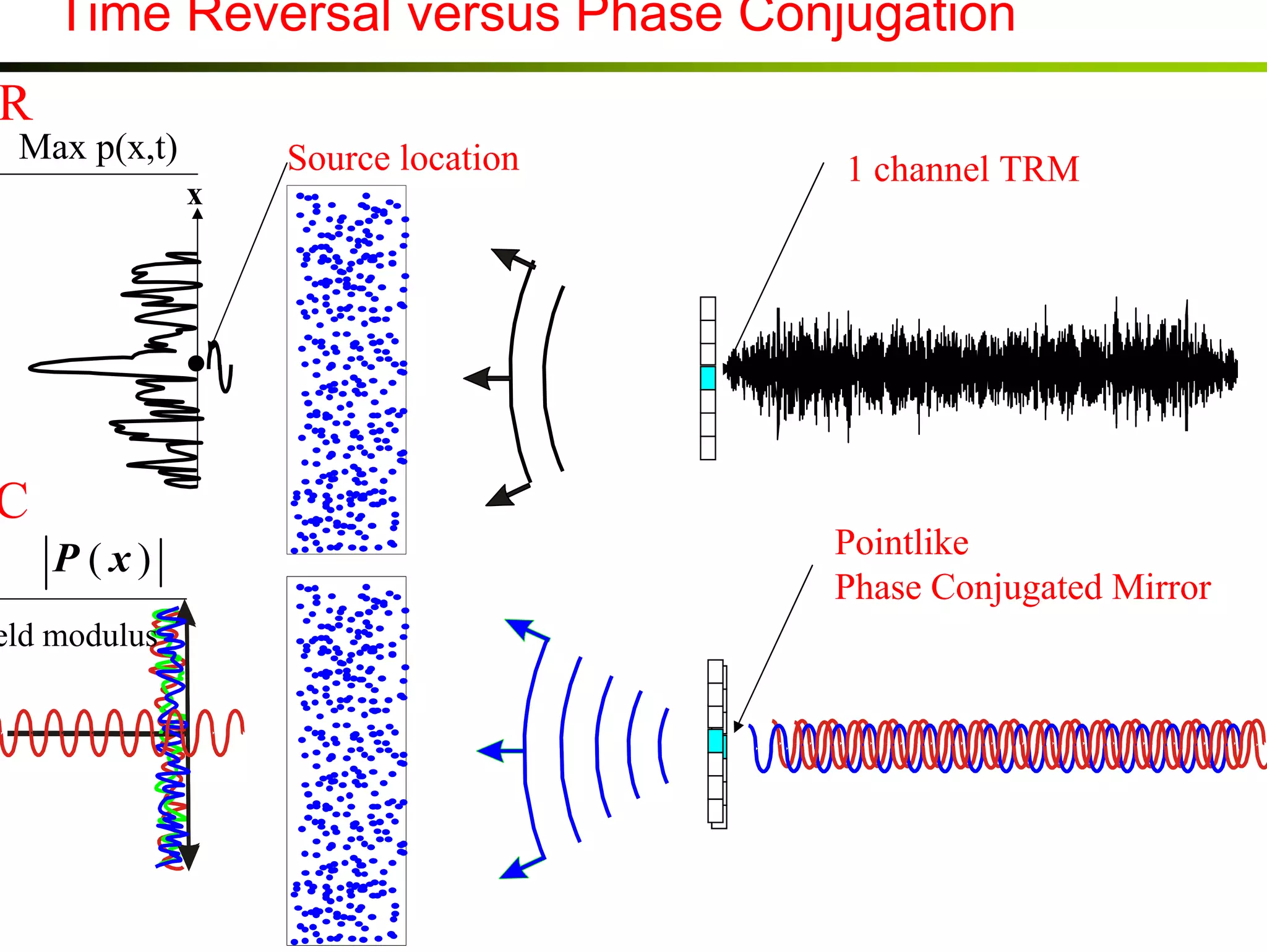
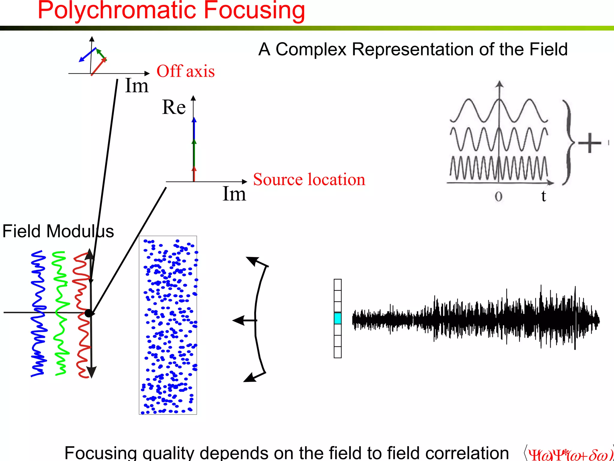
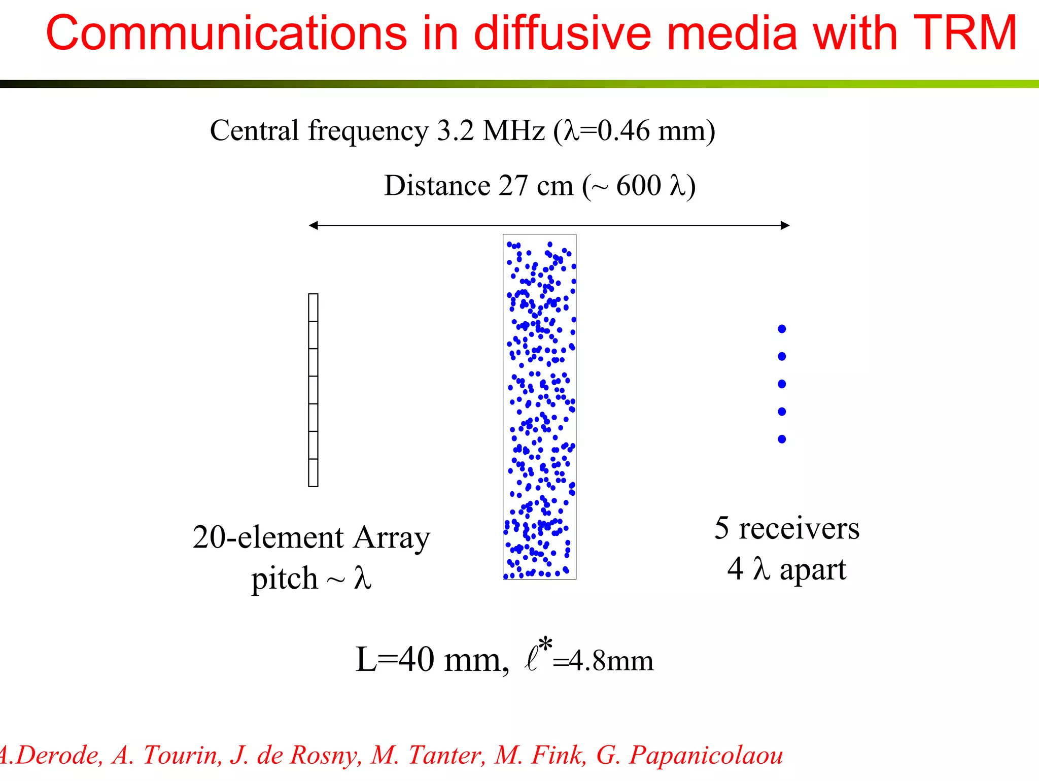
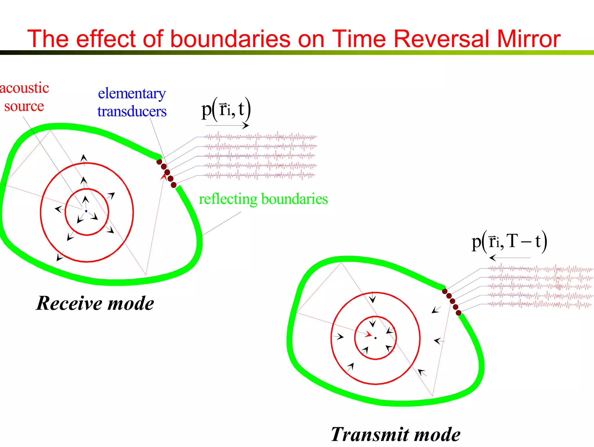
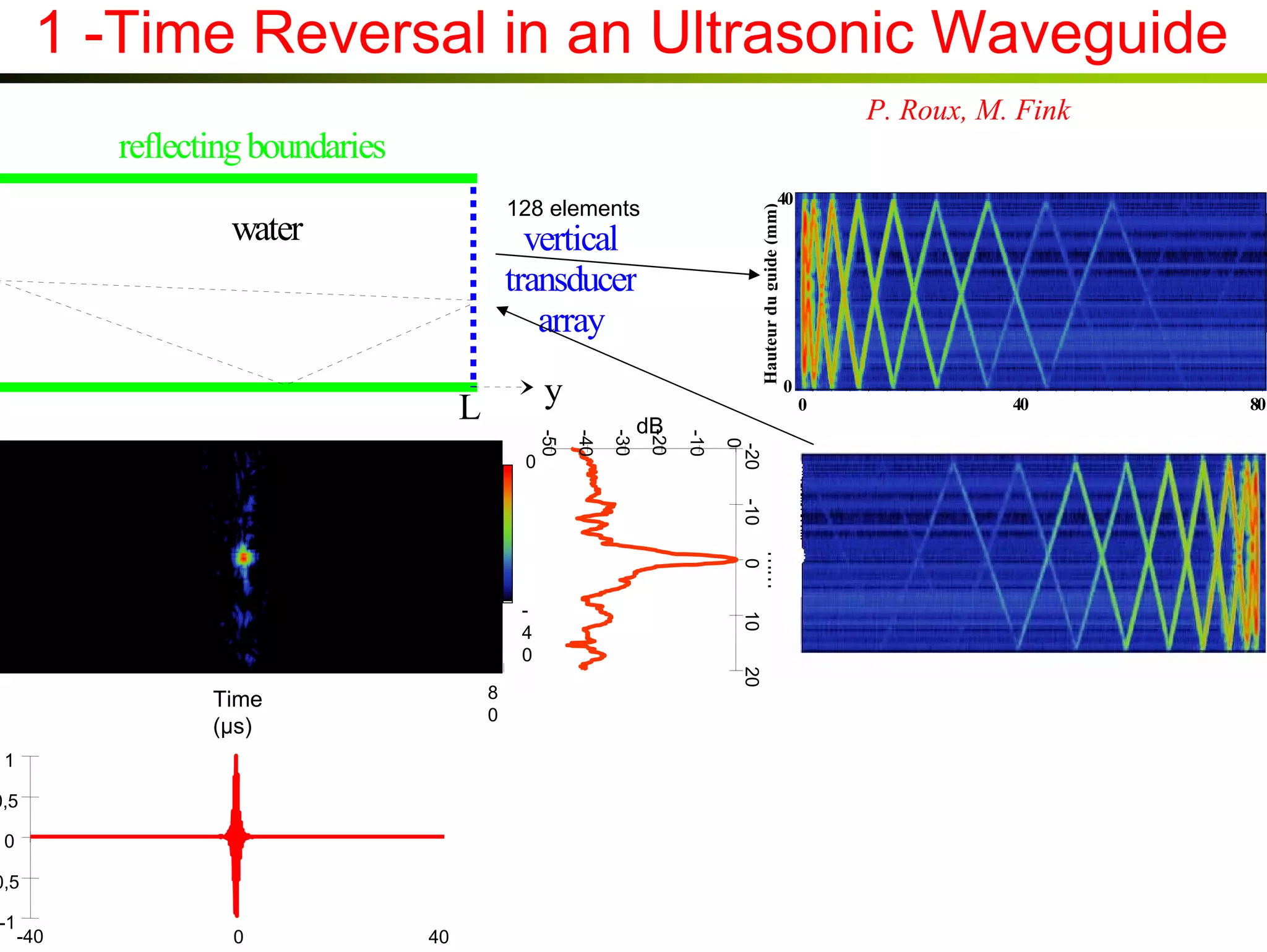
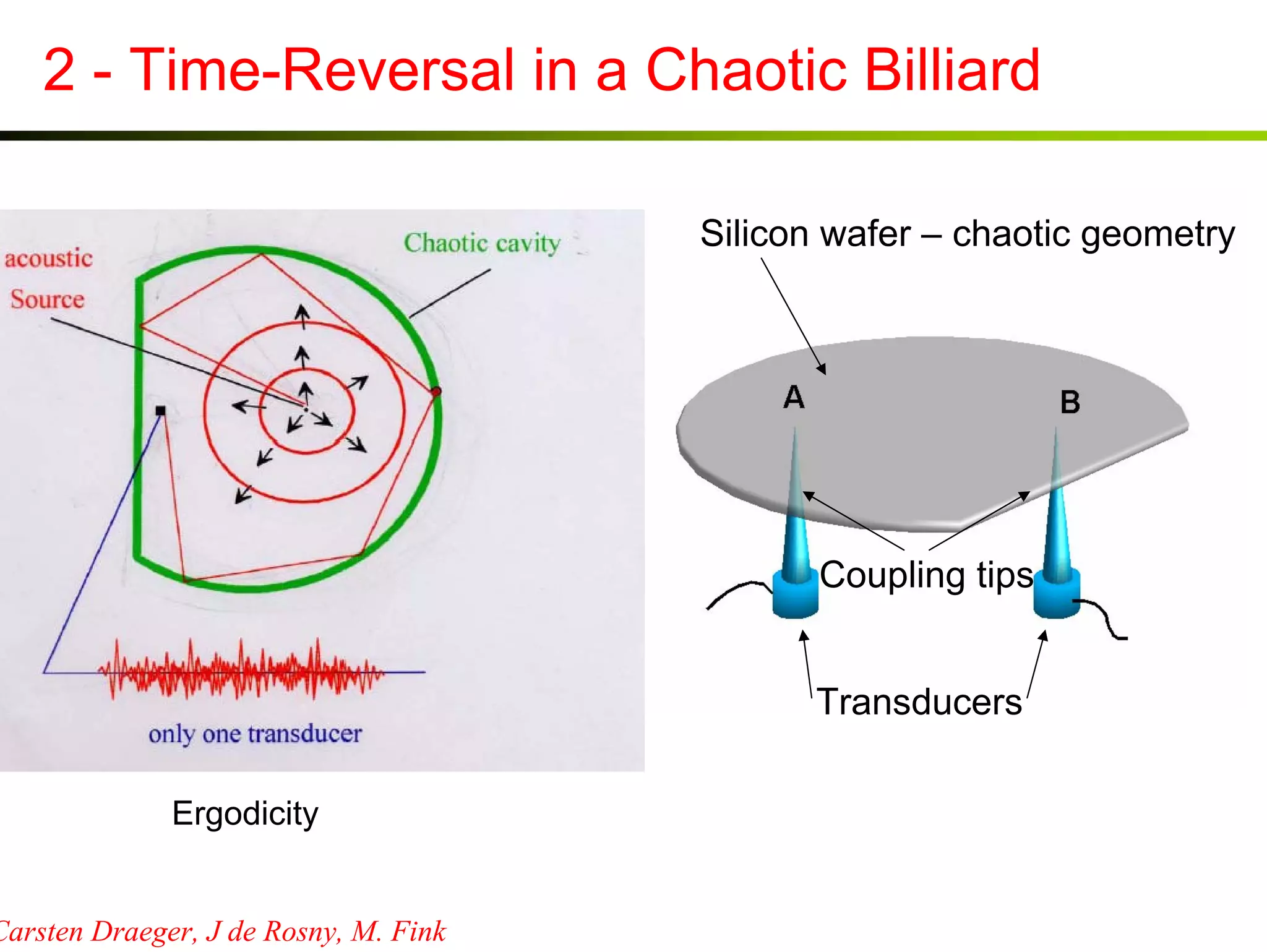
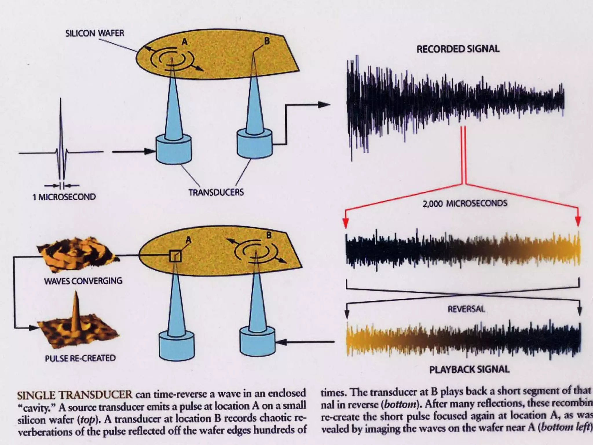
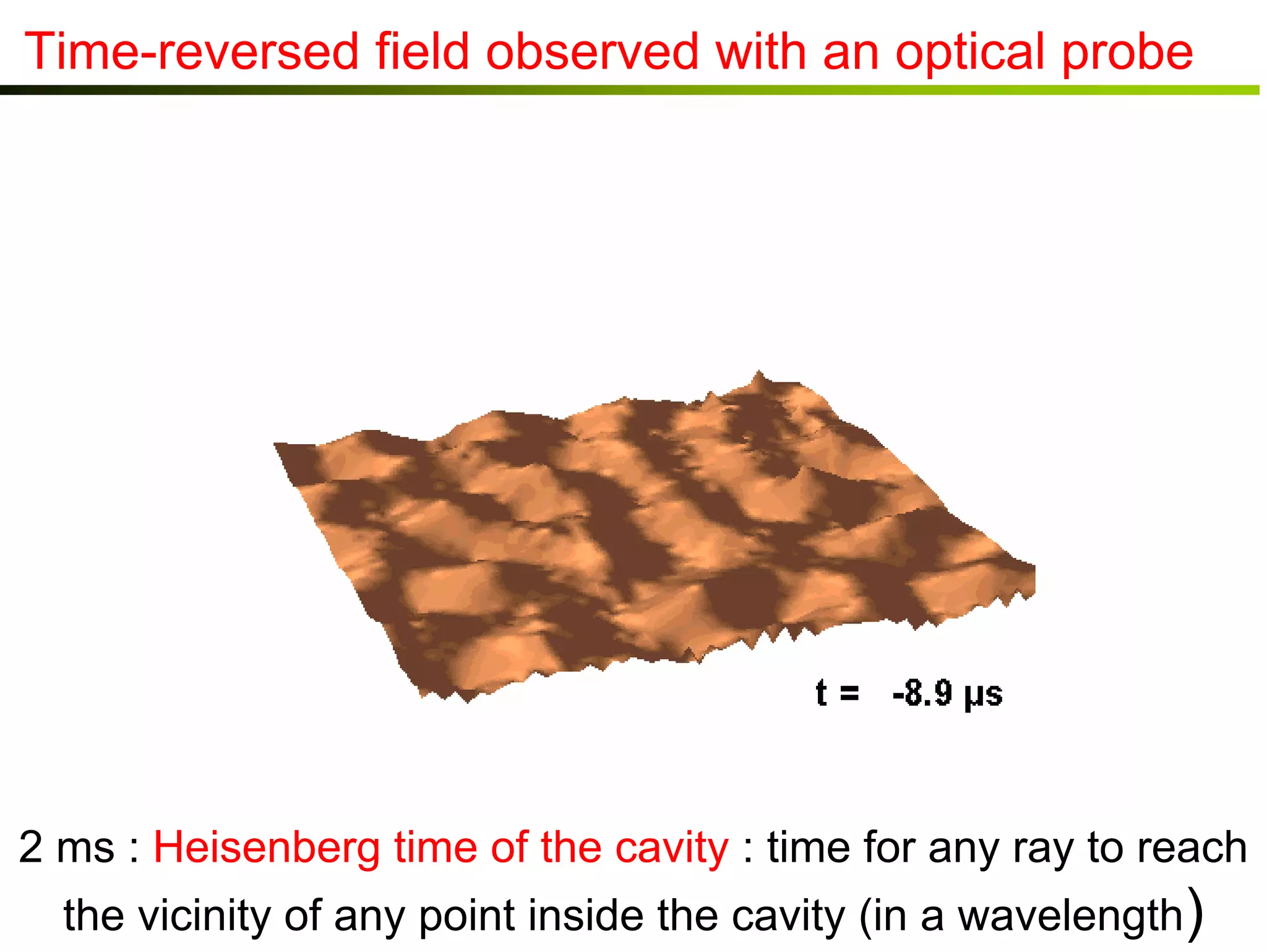
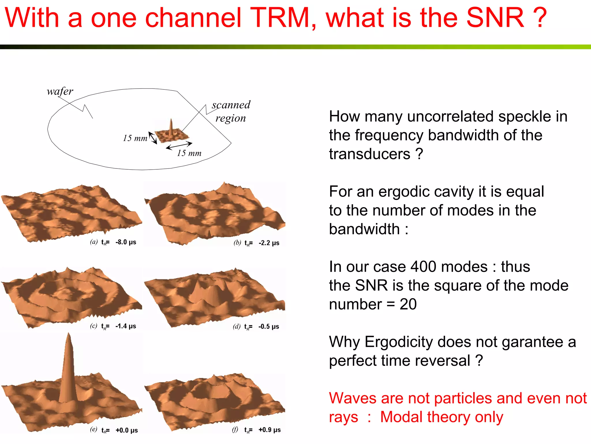
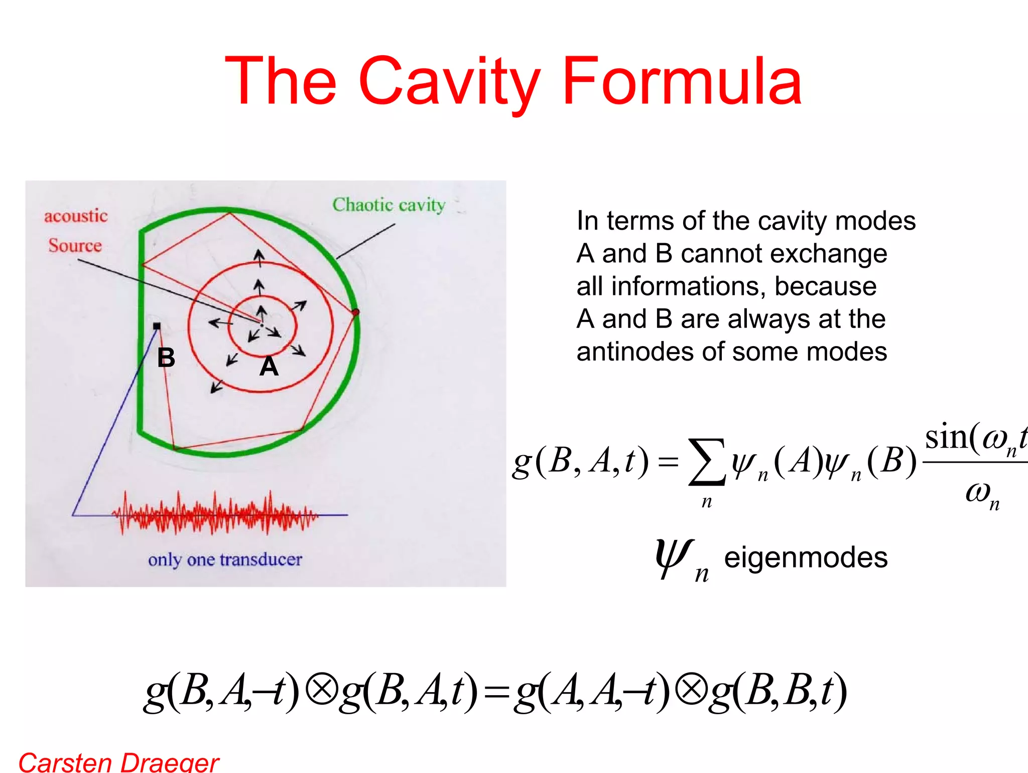
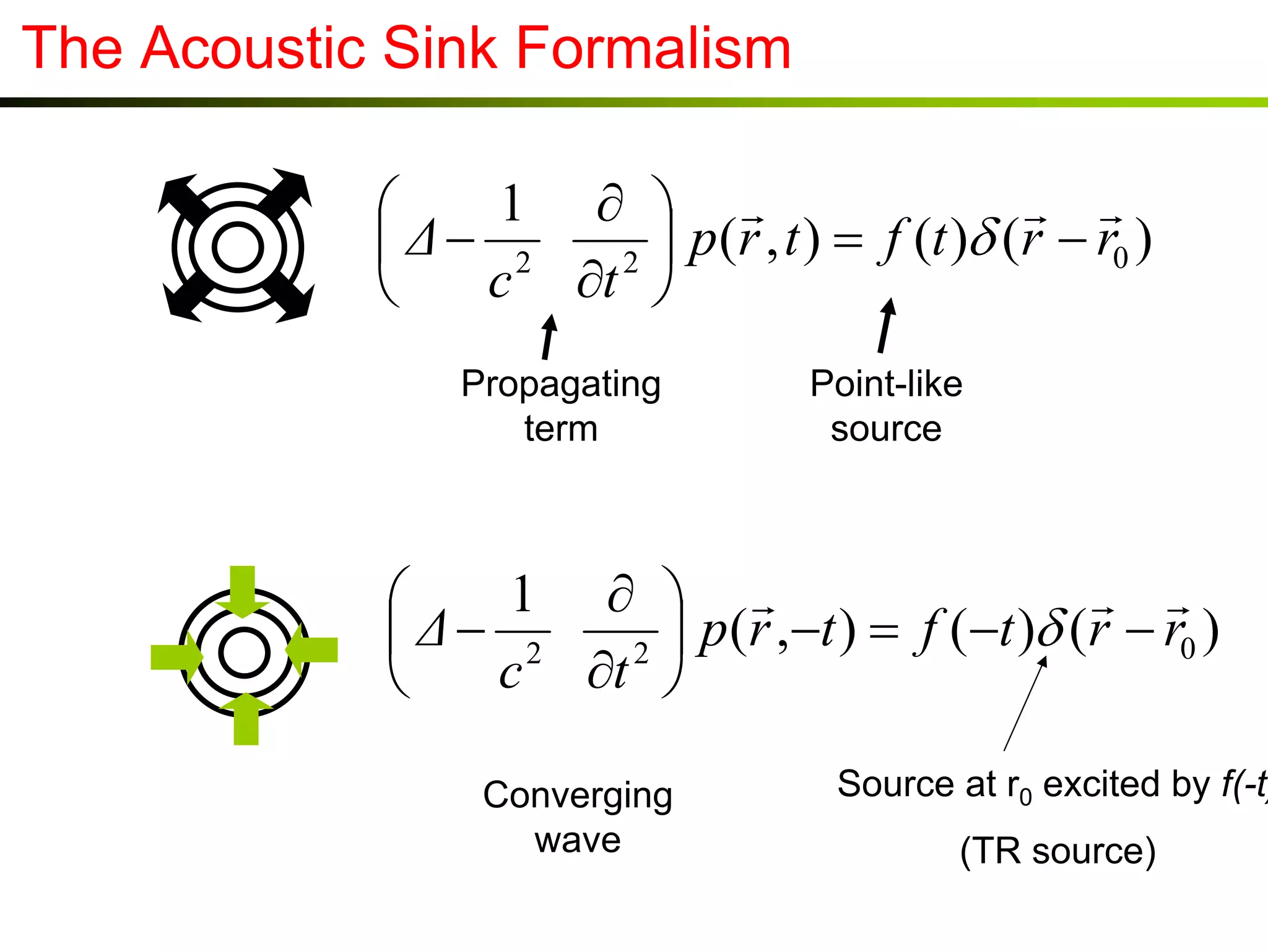
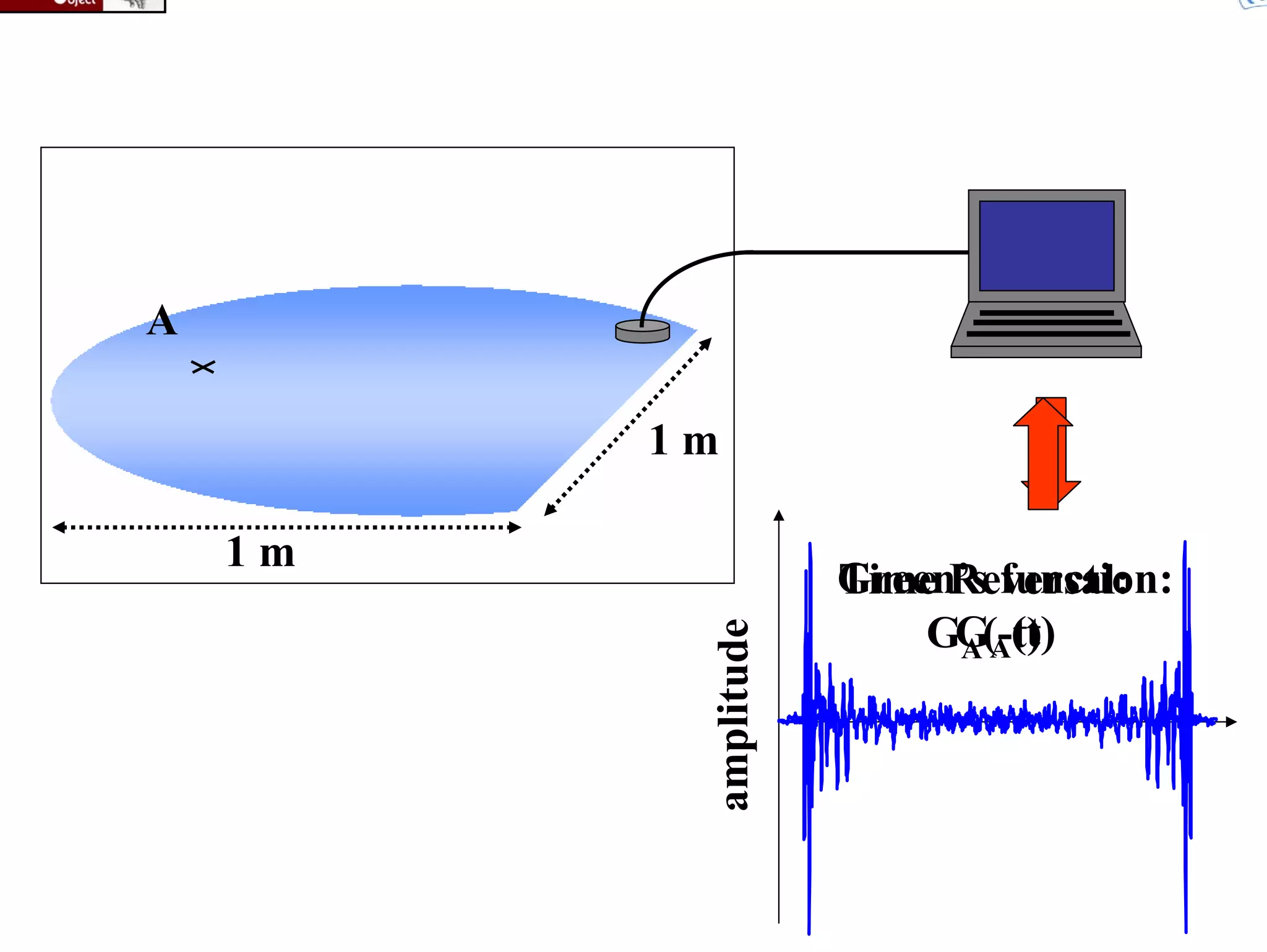
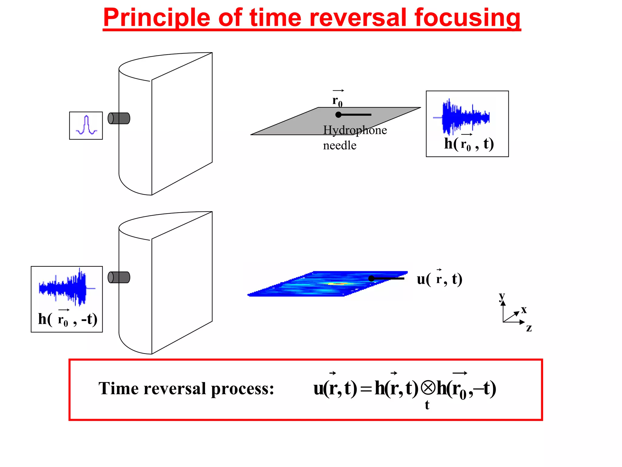
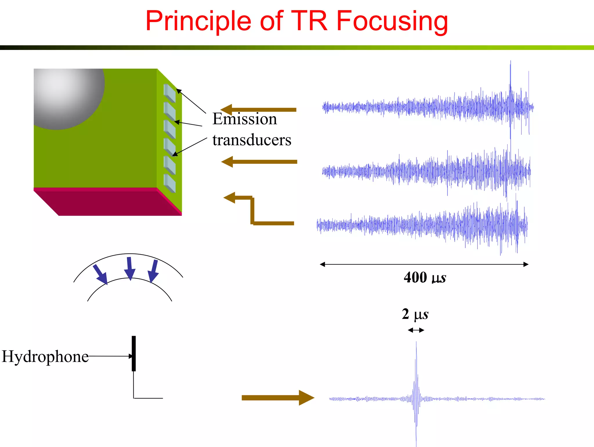
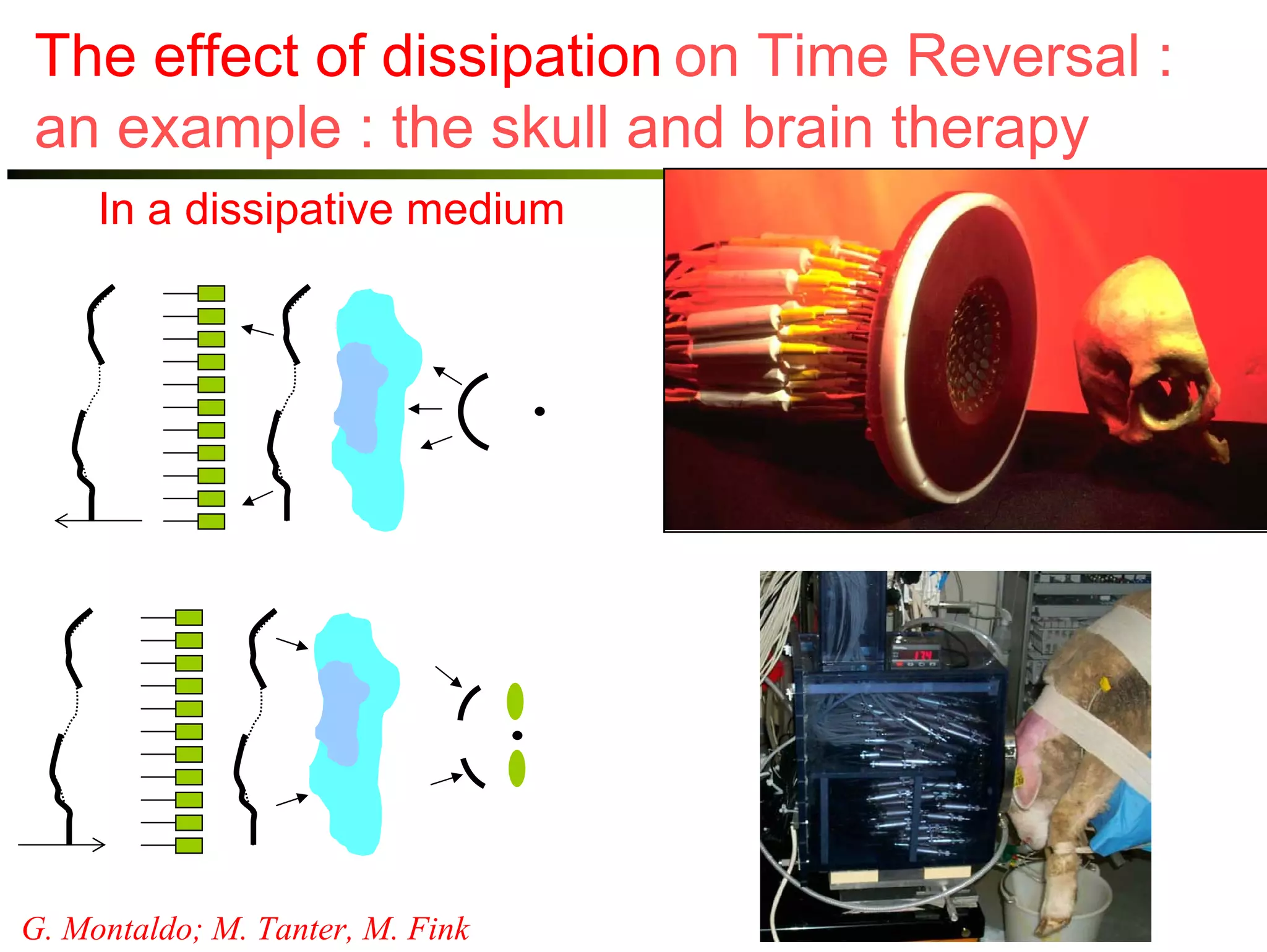
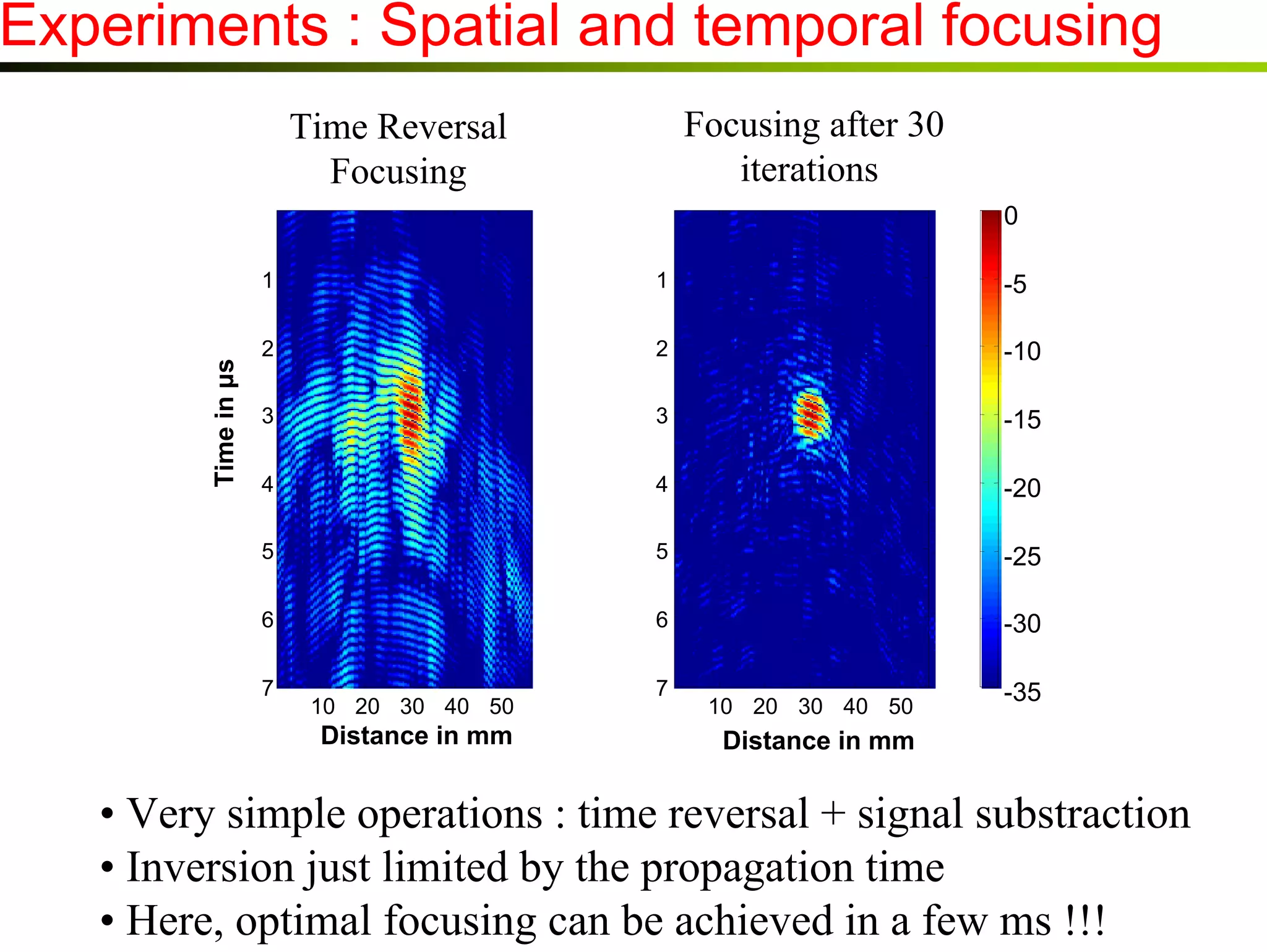
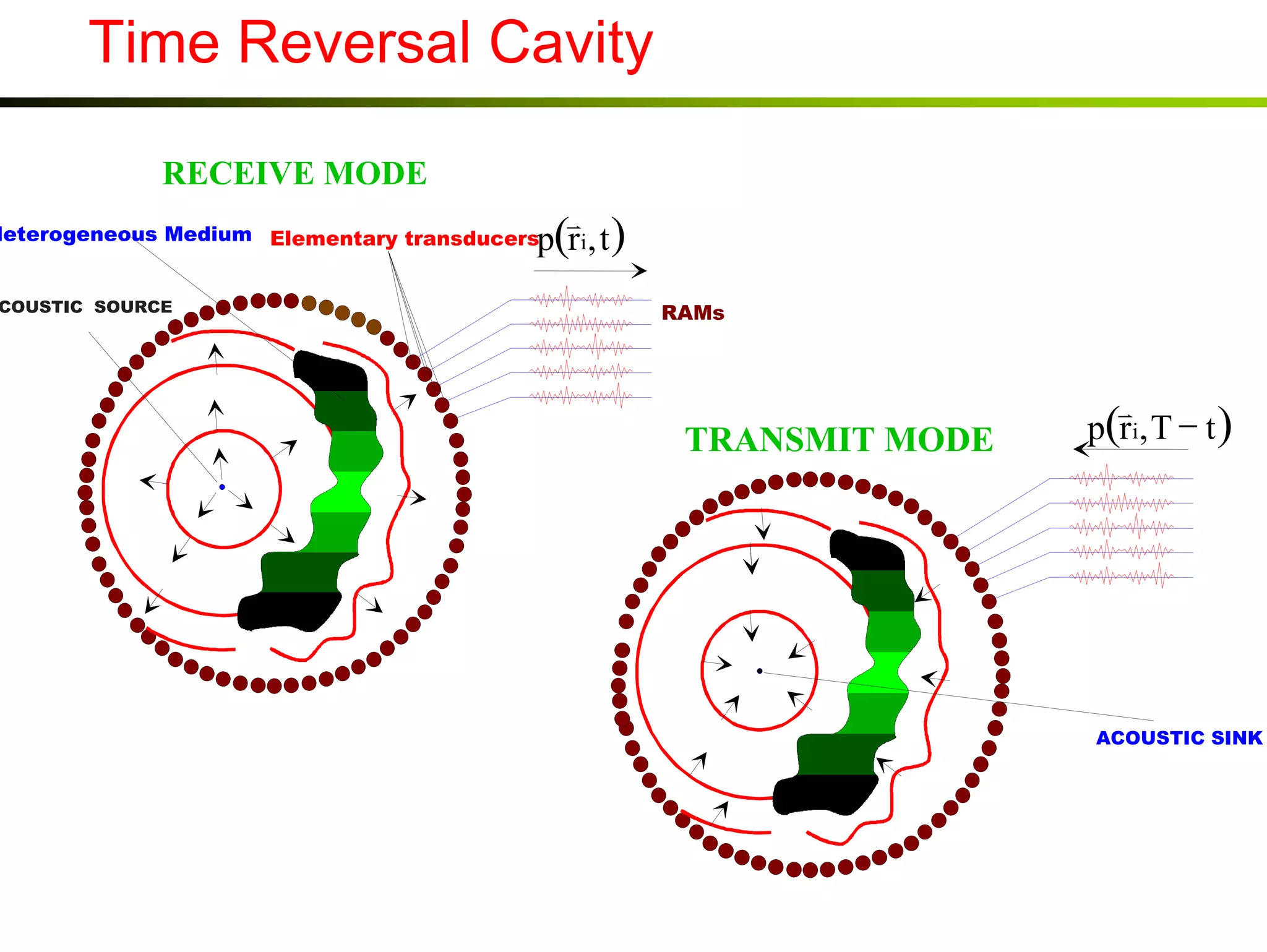
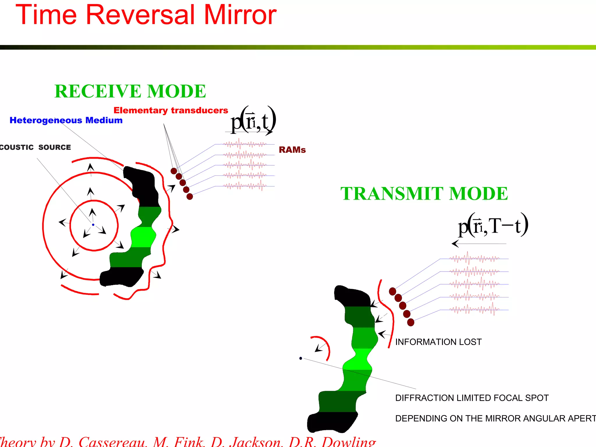
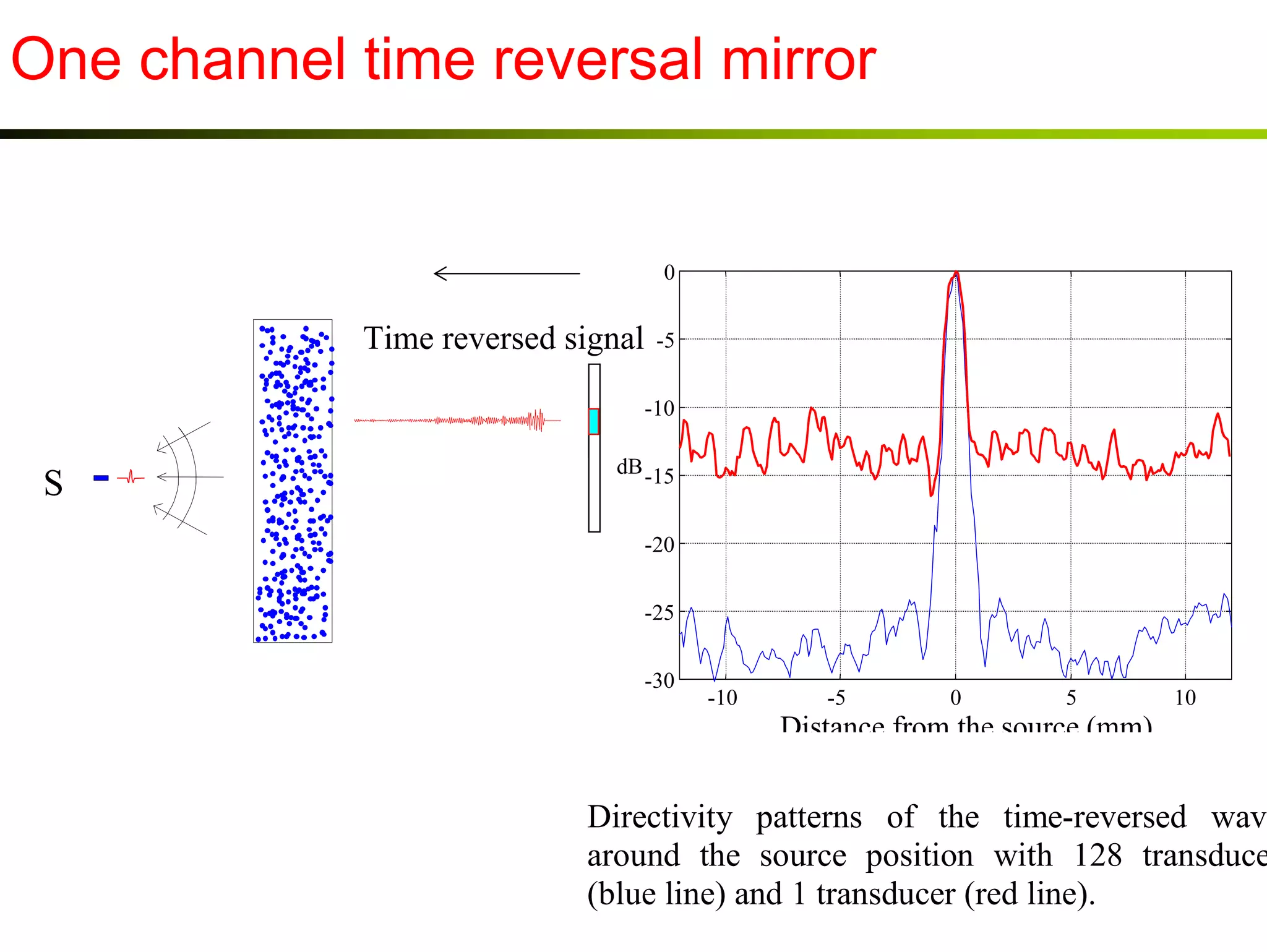
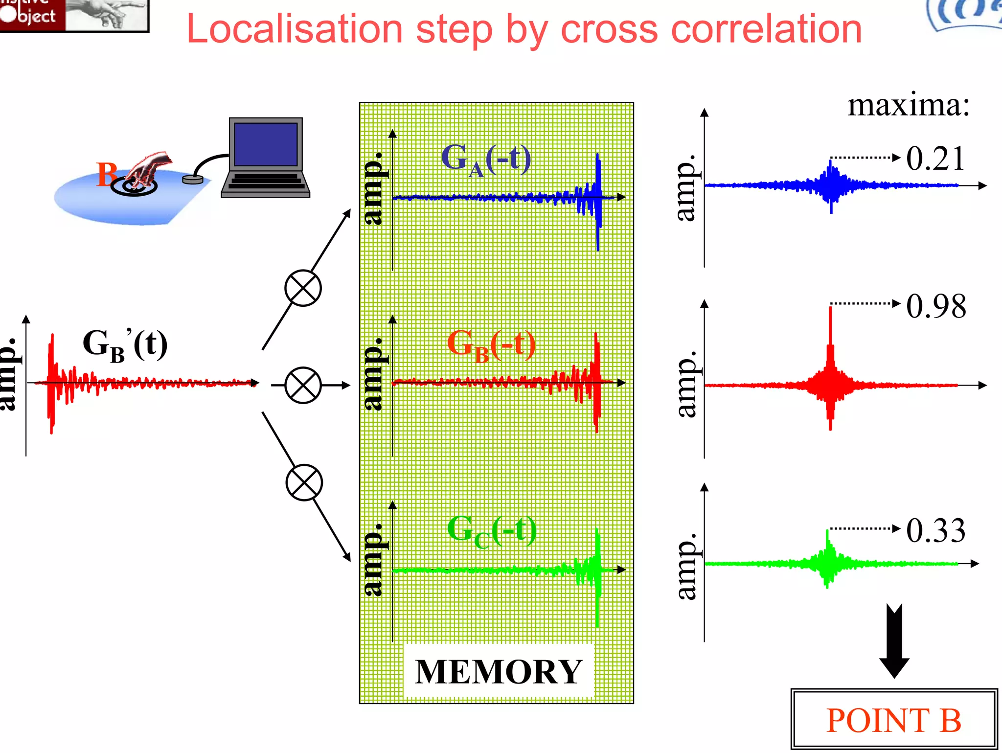
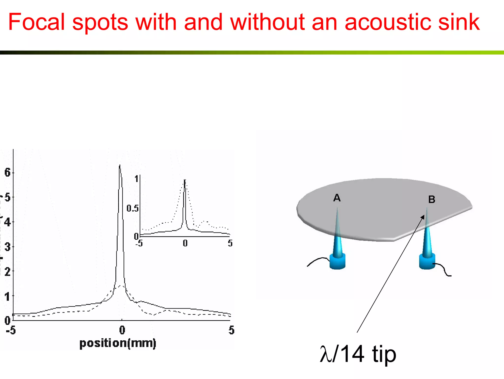
-10 -45 0 100 200 300 400 500 Time (μs) -10 -5 0 5 10 Distance (mm) 1) Time reversal acoustics utilizes the time reversal invariance of the acoustic wave equation to focus waves in space and time. 2) A time reversal mirror records acoustic waves from a source and re-emits a time-reversed version of the recorded signal to focus it back to the original source location. 3) Experiments demonstrate that time reversal focusing works in complex media like random scatterers and waveguides, achieving focusing beyond

1. Time Reversed Acoustics

2. Acoustic propagation in a non dissipative fluid
p ( r , t ) acoustic pressure field (scalar)
ρ ( r ) is the density and c ( r ) is the sound velocity in an heterogeneous medium
2
 gradp(r(r) ) 
1
∂∂2 p(r,,tt))
p(r
grad( ( p , t , t
1
div
=0
div
−−

22
22
t
ρ r
ρ r c r, p
 ρ (r ,(p))  ρ (r ,(p))c ((r ) ) ∂∂t
In NonLinear Acoustics
In Linear Acoustics
Spatial Reciprocity
Time Reversal Invariance
∂2 p ( r , t )
This equation contains only
Then if p ( r , t ) is a solution
∂t 2
t1
t0
p ( r , − t ) is also a solution
∂ p(r ,t )
2
because
∂t 2
∂ p ( r , −t )
t1
2
=
∂t 2
p( r , t )
p( r ,− t )
t0

3. Time Reversal Cavity
RECEIVE MODE
p(ri, t )
Heterogeneous Medium Elementary transducers
ACOUSTIC SOURCE
RAMs
TRANSMIT MODE
p(ri, T − t )
ACOUSTIC SINK ??

4. Time Reversal Mirror
RECEIVE MODE
Elementary transducers
Heterogeneous Medium
ACOUSTIC SOURCE
p(ri,t)
RAMs
TRANSMIT MODE
p(ri,T− t)
INFORMATION LOST
DIFFRACTION LIMITED FOCAL SPOT
DEPENDING ON THE MIRROR ANGULAR APERTURE
Theory by D. Cassereau, M. Fink, D. Jackson, D.R. Dowling

5. Time Reversal in a multiple scattering medium
TRM array
Source
Multiple scattering
medium
Time reversed signals
?
A.Derode, A. Tourin, P. Roux, M. Fink

6. The experimental setup
Linear array, 128 transducers
Acoustic source
ν=3 MHz, λ=0.5 mm
Steel rods forest
Element size ¾λ

7. Amplitude
Transmitted signal through water recorded on transducer 64
20
40
60
80
100
120
140
160
Time (µs)
Amplitude
Transmitted signal through the rods recorded on transducer 64
20
40
60
80
100
120
140
160
Time (µs)
Amplitude
Time reversed wave recorded at the source location
20
40
60
80
Time (µs)
100
120
140
160

8. Spatial focusing of the time reversed wave
Amplitude
Mobile
hydrophone
0
-5
-10
-15
-20
-25
-30 -10
- 5
0
Distance (mm)
5
10

9. One-bit versus 8-bit time reversal
8 bit time-reversal, L=40 mm
1
0.5
0
-0.5
-1
-50
-25
0
25
50
time (µs)
One-bit time reversal, L=40 mm
3
1.5
0
-1.5
-3
-50
-25
0
25
50
time (µs)
-12
-6
0
6
12 (mm)
0
-5
dB
-10
-15
-20
-25
-30
8 bit
One bit

10. One channel time reversal mirror
0
Time reversed signal
-5
-10
S
dB -15
-20
-25
-30
-10
-5
0
5
10
Distance from the source (mm)
Directivity patterns of the time-reversed waves
around the source position with 128 transducers
(blue line) and 1 transducer (red line).

11. Time Reversal versus Phase Conjugation
TR.operation → p( x, t ) ⇔ p( x,-t )
If the source is monochromatic
p( x, t ) = Re P ( x )e jω t ∝ P ( x )e jω t + P * ( x )e − jω t
with P ( x ) complex function
P ( x) = P ( x) e
jφ ( x )
Thus the TR.operation →
p( x, −t ) ∝ P ( x )e − jω t + P * ( x )e jω t
or
P ( x ) ⇔ P * ( x ),or,φ ( x ) ⇔ −φ ( x )

12. Time Reversal versus Phase Conjugation
TR
Max p(x,t)
x
Source location
1 channel TRM
.
PC
P (x)
Field modulus
Pointlike
Phase Conjugated Mirror

13. Polychromatic Focusing
A Complex Representation of the Field
Im
Off axis
Re
Im
Source location
t
Field Modulus
Focusing quality depends on the field to field correlation
Ψ(ω Ψ (ω+δω)
) *

14. How many uncorrelated speckles δω
?
FT
?
∆ω
2
2.5
3
3.5
4
4.5
5
MHz
- *
Field-field correlation Ψ(ω)Ψ ( ω+ δω = fourier transform of the travel time distribution I (t )
)
δω
FT
I (t )
0
50
Thoules time,
100
150
Time (µs)
200
δτ =D2/L ~ 150 µs
250
2
2.5
3
δω = 8 kΗz
3.5
MHz
4
4.5
5
∆ω/δω =150

15. Focusing in monochromatic mode : the lens
Spatial Diversity
λF/D
D
F

16. Spatial and Frequency Diversity
Spatial and frequency diversity
One element time reversal mirror
-5
-5
-10
TR1
0
-10
dB
0
-15
-15
PC1
-20
-20
-25
-25
-10
-5
0
5
10
-10
Phase conjugation
-5
0
5
10
Time-reversal
128 elements time reversal mirror
0
0
PC128
-5
TR128
-5
-10
-15
-15
dB
-10
-20
-20
-25
-25
-30
-30
-35
-35
-10
-5
0
5
10
-10
-5
0
5
10

17. Communications in diffusive media with TRM
Central frequency 3.2 MHz (λ=0.46 mm)
Distance 27 cm (~ 600 λ)
20-element Array
pitch ~ λ
5 receivers
4 λ apart
L=40 mm, *=4.8mm
A.Derode, A. Tourin, J. de Rosny, M. Tanter, M. Fink, G. Papanicolaou

18. Modulation BPSK
T0 = 3.5 µs
0.7µs
+1
-1
Transmission of 5 random sequences of 2000 bits to the receivers
#1
#2
#3
#4
#5
Error rate
Diffusive medium
0
0
0
1
0
10-4
Homogeneous
medium
489
640
643
602
503
28.77 %

19. Spatial focusing
12345
0
-5
-1 0
-1 5
-2 0
-2 5
-1 5
-1 0
-5
0
Diffusive medium
5
10
15
water
1
2
3
4
5
16
mm
10 µs

20. Shannon Capacity (MIMO)
C = Log2 {det (I+SNR × tH* H)} bits/s/Hz
(Cover and Thomas 1991, Foschini 1998)
Propagation Operator
hijt 
FT
H(ω)
R=HE

21. The Time Reversal Operator tH* H
array
array
HE
E
H
tH * H
E
TR
tHH*
M. Tanter
E*
tH
TR
H*E*

22. Shannon Capacity in Diffusive Media
C = Log2 {det (I+SNR × tH* H )}
H = U D V∗
T
C = Log2 {det (I+SNR × tU* D2 U )}
U t U* = I
C = Log2 {det (I+SNR × D2 )}
C=
∑Log2 {1 + SNR × λi2}
i =1.. N
N independant channels, N degrees of freedom

23. Experimental results : singular values distribution
40×40 inter-element impulse responses
Homogeneous medium
Diffusive medium
→ At 3.2 MHz : 34 / 6 singular values (–32 dB)
The number of singular values is equal to the number of
independant focal spots that one can create on the receiving
array

24. The effect of boundaries on Time Reversal Mirror
acoustic
source
elementary
transducers
p( ri, t )
reflecting boundaries
p( ri,T − t )
Receive mode
Transmit mode

25. 1 -Time Reversal in an Ultrasonic Waveguide
x
P. Roux, M. Fink
reflecting boundaries
water
S
40
128 elements
Hauteur du guide (mm)
H
vertical
transducer
array
O
y
L
-40
0
-20
0
-10
-20
-30
-40
0
-50
4
0
dB
0
Amplitude
1
0,5
0
-0,5
-1
-40
0
Time (µs)
40
20
8
0
Time
(µs)
10
0
mm
Depth
(mm)
-10
4
0
0
0
40
80µs

26. The Kaleidoscopic Effect : Virtual Transducers
mm
Amplitude (dB)
-20
-10
0
10
20
0
Open space
-10
Waveguide effect
-20
-30
-40
-50
guide d'onde
eau libre
A comparison between the focal spot with and without the waveguide
TRM
image
point S
source
real
TRM
aperture
aperture
of the TRM
of the TRM
in the
in free water waveguide
If the pitch is to large : grating lobes

27. Time Reversal in Ocean Acoustics
B. Kuperman, SCRIPPS
3.5 kHz SRA (’99 and ’00)
L = 78 m
N = 29
3.5 kHz tranceiver

28. Up-slope Experiment: Elba
10 km
30 m
100 m
1m
Diffraction limit

29. 2 - Time-Reversal in a Chaotic Billiard
Silicon wafer – chaotic geometry
Coupling tips
Transducers
Ergodicity
Carsten Draeger, J de Rosny, M. Fink

31. Time-reversed field observed with an optical probe
2 ms : Heisenberg time of the cavity : time for any ray to reach
the vicinity of any point inside the cavity (in a wavelength)

32. With a one channel TRM, what is the SNR ?
wafer
scanned
region
15 mm
15 mm
How many uncorrelated speckle in
the frequency bandwidth of the
transducers ?
For an ergodic cavity it is equal
to the number of modes in the
bandwidth :
(a)
R
(b)
R
In our case 400 modes : thus
the SNR is the square of the mode
number = 20
(c)
R
(d)
R
Why Ergodicity does not garantee a
perfect time reversal ?
(e)
R
(f)
Waves are not particles and even not
rays : Modal theory only
R

33. The Cavity Formula
B
A
In terms of the cavity modes
A and B cannot exchange
all informations, because
A and B are always at the
antinodes of some modes
g ( B, A, t ) = ∑ψ n ( A)ψ n ( B )
n
ψ n eigenmodes
g(B, A,−t) ⊗g(B, A,t) = g(A, A,−t) ⊗g(B, B,t)
Carsten Draeger
sin(ωn t )
ωn

34. Origin of the diffraction limit
Wave focusing : 3 steps
Converging only
Monochromatic
exp {j(kr+ωt)} / r
with singularity
J. de Rosny, M. Fink
Both converging
and diverging
waves interfere
Sin (kr)/r . exp(jωt)
without singularity
Diffraction limit
(λ/2)
Diverging only
exp {j(-kr+ωt)} / r
with singularity

35. « Perfect » TR - the acoustic sink
Goal
converging
No interference
and singularity
exp {j(kr+ωt)} / r
No diffraction
limit
with singularity

36. Principle of the acoustic sink
Out of phase

37. The Acoustic Sink Formalism
1 ∂ 

p (r , t ) = f (t )δ (r − r0 )
 ∆− 2
2 
c ∂t 

Propagating
term
Point-like
source
1 ∂ 

p (r ,−t ) = f (−t )δ (r − r0 )
 ∆− 2
2 
c ∂t 

Converging
wave
Source at r0 excited by f(-t)
(TR source)

39. Focal spots with and without an acoustic sink
λ/14 tip

40. A nice application of Chaos : Interactive Objects
How to transform any object in a tactile screen ?
accelerometer
100Hz <∆Ω < 10kHz
A
1m
amplitude
1m
R. Ing, N. Quieffin, S. Catheline, M. Fink
Green’s function:
GA(t)
time

41. A
1m
amplitude
1m
Green’s function:
Time Reversal:
GG(-t)
A A(t)

42. amp.
amp.
B
A
GA(t)
GB(t)
amp.
Training step: library of Green functions
GC(t)
10ms
10ms
C
10ms
MEMORY

43. Localisation step by cross correlation
GC(-t)
amp.
amp.
GB(-t)
0.21
0.98
amp.
amp.
GB’(t)
GA(-t)
amp.
amp.
B
amp.
maxima:
0.33
MEMORY
POINT B

44. Tactile Objects

45. Some other examples

46. Time Reversal in Leaky Cavities and
Waveguides
• A new concept of smart transducer design
with reverberation and programmable
transmitters
• What happens if the source is outside the
waveguide ?

47. A first example : the D shape billiard
contact transducer
half-cylinder
hydrophone needle

48. Principle of time reversal focusing
r0
Hydrophone
needle
h( r0 , t)
u( r , t)
y
h( r0 , -t)
Time reversal process:
u(r, t) = h(r, t) ⊗h(r0 ,−t)
t
x
z

49. Time Reversal Focusing with steering
contact
transducer
130mm
moving pulsed source
y
100m
m
Abscissa x (mm)
-25
0
25
75
100
Time of arrival
125
x
z

50. A second example : the SINAI BILLIARD
z
x
30 emission
transducers
(1.5 MHz ,
5mm x 8 mm
pitch 1 mm)
Large transducer
element, not optimized
y
Motors
hydrophone
electronics
Electronics :
Fully programmable multi-channel
system.

51. Principle of TR Focusing
Emission
transducers
400 µs
2 µs µs
2
Hydrophone

52. (Fundamental and Harmonics)
dB 0
0.8
-5
Distance(mm)
0.6
Amplitude
FUNDAMENTAL
TR Kaleidoscope
0.4
0.2
0
-15
-25
-35
-0.2
-0.4
0
Spatial lobes : - 30 dB
Temporal lobes : - 38 dB
20
40
60
80
100
Time (µs)
-45
Distance(mm)
dB 0
0.6
Distance(mm)
Amplitude
HARMONIC
-5
0.4
0.2
0
-0.2
-15
-25
-35
-0.4
0
Temporal lobes : -60 dB 100
20
40
60
80
Time (µs)
Spatial Lobes ~ - 50 dB
Distance(mm)
-45

53. Building a 3D Image
Reception
transducer
(harmonic)
Distance (mm)
Emission
transducers
0
-20
-40
-60
-80
40
40
Object
20
Distance (mm)
20
0 0
Distance (mm)

54. The effect of dissipation on Time Reversal :
an example : the skull and brain therapy
In a dissipative medium
G. Montaldo; M. Tanter, M. Fink

55. Influence of the trabecular bone on the acoustic
propagation
Diploë :Porous zone
(c = 2700 m.s 1)
External wall
(c = 3000 m.s 1)
Internal wall
(c = 3000 m.s 1)
2
 grad p ( r , t ) 
∂ 
1 ∂ p (r , t )

−
=0
 1 +τ ( r )  ρ ( r ) div 


2
2
∂t 
ρ (r )

∂t

 c (r )
Breaking the time reversal invariance

56. The iterative method
o(-t)
o(t)+d(t)
d(t)
d(t)+d(t)
o(t)-d(t)
e(t)
e(-t)
c(t)
First transmit step :
the objective
T.R and reemission :
reconstruction of the
objective
Emission of the
lobes
Lobes reconstruction
c(-t)
e(-t)-c(-t)
The difference
eliminates the lobes

57. Experiments : improvement of the focal spot
Water
128 elts.
1.5 MHz
Pitch 0.5 mm
Absorbing
And aberrating
Ureol sample
128 elts.
1.5 MHz
Pitch 0.5 mm
F = 60 mm
0
-5
Amplitude in Db
-10
-15
-20
1
-25
10
-30
20
-35
30
-40
-45
0
10
20
30
40
Distance in mm
50
60
D = 60 mm

58. Experiments : Spatial and temporal focusing
Focusing after 30
iterations
Time Reversal
Focusing
0
1
-5
2
2
-10
3
3
-15
4
4
-20
5
5
-25
6
Time in µs
1
6
-30
7
10 20 30 40 50
Distance in mm
7
10 20 30 40 50
-35
Distance in mm
• Very simple operations : time reversal + signal substraction
• Inversion just limited by the propagation time
• Here, optimal focusing can be achieved in a few ms !!!

59. Focusing through the Skull
Classical Cylindrical law
Optimal signal to transmit
2
51
0
Transducer
number j
2
12 5 1
8
Spatial focusing
0
Transducer
number j
-5
Pressure (dB)
0
-10
-15
-20
-25
-30
-35
-20
-10
0
10
20
Distance from the initial point source
(mm)

60. 300 elements Time Reversal Mirror (Therapy/Imaging)
Global view
(300 elements and C 4-2 echographic probe)
Front view
(300 elements and C 4-2 echographic probe)
Coupling + cooling system
128 Channels of a HDI 1000 scanner
200 Emission boards for THERAPY
Spherical active surface:
Aperture 180 mm
Focal dist. 140 mm
100 Emission/Reception boards for THERAPY+IMAGING

61. Correction of skull aberrations using an implanted hydrophone
Experimental scan
without correction
Experimental scan
with correction
(Time reversal + Amplitude
Compensation)
Acoustic Pressure measured at focus : - 70 Bars, 1600 W.cm-2 (with correction)
- 15 Bars, 80 W.cm-2 (without correction)

62. Transkull in vivo experiments

63. Transkull in vivo experiments
MRI
Histology
Transkull in vivo thermally induced necrosis