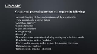
Download as PDF, PPTX

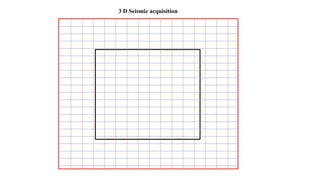
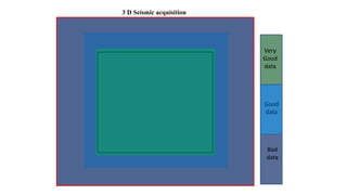
![Seismic acquisition
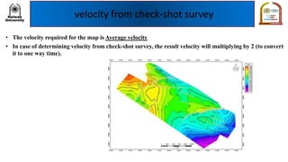
• Example 1:
V = 7,000 m/s
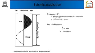
F = 50 Hz
l= V/F
= 7,000/50
[(m/s)/(cycles/s)]
= …….m
• Example 2:
V = 3,000 m/s
F = 50 Hz
l= V/F
= 3,000/50 [(m/s)/(cycles/s)]
= ……….m](https://image.slidesharecdn.com/introductiontoseismicinterpretation-171126161353/85/Introduction-to-seismic-interpretation-20-320.jpg)
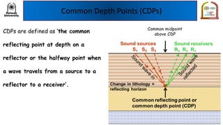
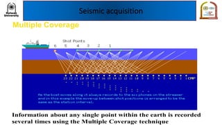


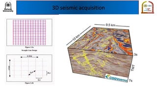
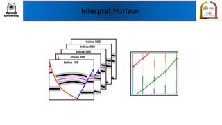


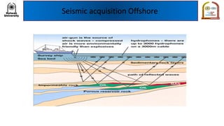
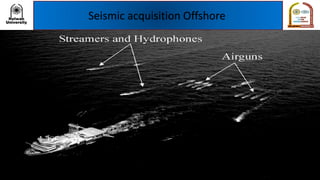
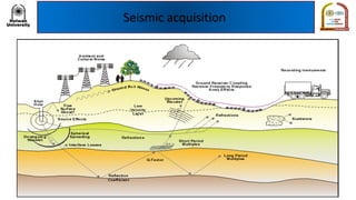
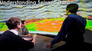
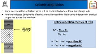
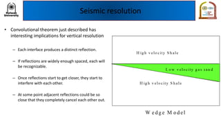
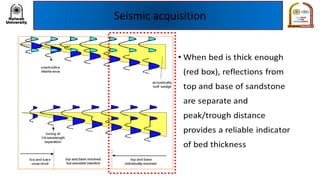
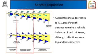
This document provides an introduction to seismic interpretation. It begins with an overview of seismic acquisition methods both onshore and offshore. It then discusses key concepts in seismic data such as common depth points, floating datum, two-way time, and the relationship between time and depth. The document also covers seismic resolution, reflection coefficients, and examples of calculating tuning thickness. Finally, it discusses important steps for seismic interpretation including checking the line scale and orientation and interpreting major reflectors and geometries.


