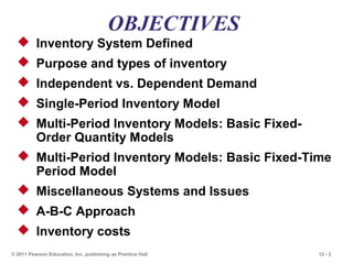
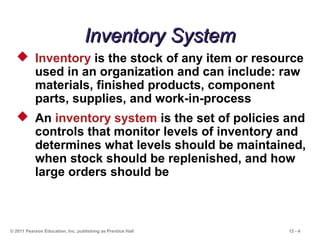
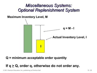
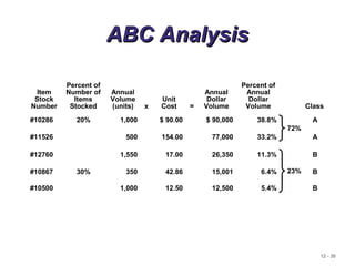
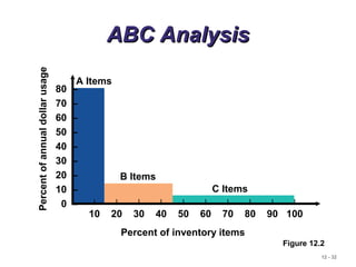
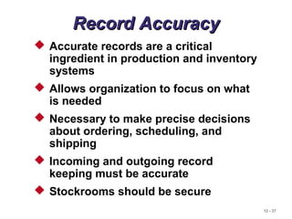
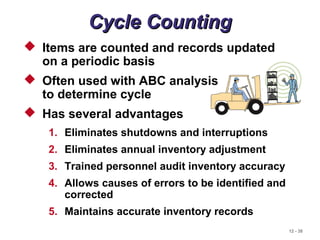
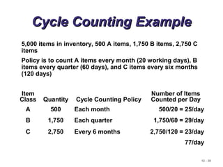
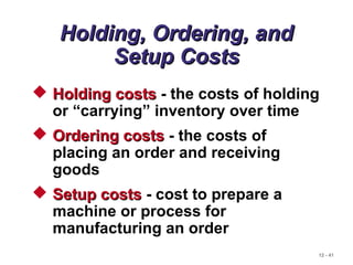
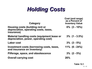
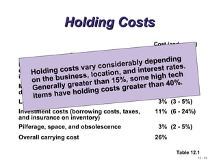
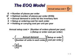
The document discusses inventory control systems, including the purpose and types of inventory, demand types, and various inventory models such as single-period and multi-period models. It also covers inventory management objectives, costs associated with holding, ordering, and setup, as well as approaches like ABC analysis and cycle counting for inventory accuracy. Additionally, the document highlights the importance of balancing inventory investment with customer service.

1. 12 - 1
Inventory Control

2. 12 - 2
OBJECTIVES
© 2011 Pearson Education, Inc. publishing as Prentice Hall
 Inventory System Defined
 Purpose and types of inventory
 Independent vs. Dependent Demand
 Single-Period Inventory Model
 Multi-Period Inventory Models: Basic Fixed-
Order Quantity Models
 Multi-Period Inventory Models: Basic Fixed-Time
Period Model
 Miscellaneous Systems and Issues
 A-B-C Approach
 Inventory costs

3. 12 - 3
OBJECTIVES
© 2011 Pearson Education, Inc. publishing as Prentice Hall
 Basic EOQ models
 EOQ examples
 ROP and it’s examples
 Production order quantity model
 Quantity discount models and examples
 Probabilistic models and safety stock
 Safety stock and probabilistic examples

4. 12 - 4
Inventory SystemInventory System
© 2011 Pearson Education, Inc. publishing as Prentice Hall
 Inventory is the stock of any item or resource
used in an organization and can include: raw
materials, finished products, component
parts, supplies, and work-in-process
 An inventory system is the set of policies and
controls that monitor levels of inventory and
determines what levels should be maintained,
when stock should be replenished, and how
large orders should be

5. 12 - 5
Purposes of InventoryPurposes of Inventory
© 2011 Pearson Education, Inc. publishing as Prentice Hall
1. To maintain independence of operations
2. To meet variation in product demand
3. To allow flexibility in production
scheduling
4. To provide a safeguard for variation in raw
material delivery time
5. To take advantage of economic purchase-
order size

6. 12 - 6
Types of InventoryTypes of Inventory
 Raw material
 Purchased but not processed
 Work-in-process
 Undergone some change but not completed
 A function of cycle time for a product
 Maintenance/repair/operating (MRO)
 Necessary to keep machinery and
processes productive
 Finished goods
 Completed product awaiting shipment

7. 12 - 7
Types of InventoryTypes of Inventory
© 2011 Pearson Education, Inc. publishing as Prentice Hall

8. 12 - 8
The Material Flow CycleThe Material Flow Cycle
Figure 12.1
Input Wait for Wait to Move Wait in queue Setup Run Output
inspection be moved time for operator time time
Cycle time
95% 5%

9. 12 - 9
Independent vs. DependentIndependent vs. Dependent
DemandDemand
© 2011 Pearson Education, Inc. publishing as Prentice Hall
Independent Demand (Demand for the final end-
product or demand not related to other items)
Finished
product
Dependent
Demand
(Derived demand
items for
component
parts,
subassemblies,
raw materials,
etc)
Component parts

10. 12 - 10
Inventory SystemsInventory Systems
© 2011 Pearson Education, Inc. publishing as Prentice Hall
 Single-Period Inventory Model
 One time purchasing decision (Example:
vendor selling t-shirts at a football game)
 Seeks to balance the costs of inventory
overstock and under stock
 Multi-Period Inventory Models
 Fixed-Order Quantity Models
 Event triggered (Example: running out of
stock)
 Fixed-Time Period Models
 Time triggered (Example: Monthly sales
call by sales representative)

11. 12 - 11
Single-Period Inventory ModelSingle-Period Inventory Model
© 2011 Pearson Education, Inc. publishing as Prentice Hall
uo
u
CC
C
P
+
≤
soldbeunit willy that theProbabilit
estimatedunderdemandofunitperCostC
estimatedoverdemandofunitperCostC
:Where
u
o
=
=
=
P
This model states that we
should continue to increase
the size of the inventory so
long as the probability of
selling the last unit added is
equal to or greater than the
ratio of: Cu/Co+Cu
This model states that we
should continue to increase
the size of the inventory so
long as the probability of
selling the last unit added is
equal to or greater than the
ratio of: Cu/Co+Cu

12. 12 - 12© 2011 Pearson Education, Inc. publishing as Prentice Hall

13. 12 - 13© 2011 Pearson Education, Inc. publishing as Prentice Hall

14. 12 - 14© 2011 Pearson Education, Inc. publishing as Prentice Hall

15. 12 - 15© 2011 Pearson Education, Inc. publishing as Prentice Hall

16. 12 - 16© 2011 Pearson Education, Inc. publishing as Prentice Hall

17. 12 - 17© 2011 Pearson Education, Inc. publishing as Prentice Hall

18. 12 - 18© 2011 Pearson Education, Inc. publishing as Prentice Hall

19. 12 - 19
Single Period Model ExampleSingle Period Model Example
© 2011 Pearson Education, Inc. publishing as Prentice Hall
 Our college basketball team is playing in a
tournament game this weekend. Based on our
past experience we sell on average 2,400 shirts
with a standard deviation of 350. We make $10
on every shirt we sell at the game, but lose $5
on every shirt not sold. How many shirts should
we make for the game?
Cu = $10 and Co = $5; P ≤ $10 / ($10 + $5) = .667
Z.667 = .432 (use NORMSDIST(.667) or Appendix E)
therefore we need 2,400 + .432(350) = 2,551 shirts

20. 12 - 20
Fixed-Period (P) SystemsFixed-Period (P) Systems
 Orders placed at the end of a fixed period
 Inventory counted only at end of period
 Order brings inventory up to target level
 Only relevant costs are ordering and holding
 Lead times are known and constant
 Items are independent from one another

21. 12 - 21
Fixed-Period (P) ExampleFixed-Period (P) Example
Order amount (Q) = Target (T) - On-
hand inventory - Earlier orders not yet
received + Back orders
Q = 50 - 0 - 0 + 3 = 53 jackets
3 jackets are back ordered No jackets are in stock
It is time to place an order Target value = 50

22. 12 - 22
Fixed-Period SystemsFixed-Period Systems
 Inventory is only counted at each
review period
 May be scheduled at convenient times
 Appropriate in routine situations
 May result in stockouts between
periods
 May require increased safety stock

23. 12 - 23
Multi-Period Models:Multi-Period Models:
Fixed-Order Quantity Model AssumptionsFixed-Order Quantity Model Assumptions
© 2011 Pearson Education, Inc. publishing as Prentice Hall
 Demand for the product is constant
and uniform throughout the period
 Lead time (time from ordering to
receipt) is constant
 Price per unit of product is constant

24. 12 - 24© 2011 Pearson Education, Inc. publishing as Prentice Hall
 Ordering or setup costs are constant
 All demands for the product will be
satisfied (No back orders are allowed)

25. 12 - 25
Miscellaneous Systems:Miscellaneous Systems:
Optional Replenishment SystemOptional Replenishment System
© 2011 Pearson Education, Inc. publishing as Prentice Hall
Maximum Inventory Level, M
Actual Inventory Level, I
q = M - I
I
Q = minimum acceptable order quantity
If q > Q, order q, otherwise do not order any.

26. 12 - 26
Miscellaneous Systems:Miscellaneous Systems:
Bin SystemsBin Systems
© 2011 Pearson Education, Inc. publishing as Prentice Hall
Two-Bin System
Full Empty
Order One Bin of
Inventory
One-Bin System
Periodic Check
Order Enough to
Refill Bin

27. 12 - 27
Inventory ManagementInventory Management
The objective of inventoryThe objective of inventory
management is to strike a balancemanagement is to strike a balance
between inventory investment andbetween inventory investment and
customer servicecustomer service

28. 12 - 28
Managing InventoryManaging Inventory
1. How inventory items can be
classified
2. How accurate inventory records
can be maintained

29. 12 - 29
ABC AnalysisABC Analysis
 Divides inventory into three classes
based on annual dollar volume
 Class A - high annual dollar volume
 Class B - medium annual dollar
volume
 Class C - low annual dollar volume
 Used to establish policies that
focus on the few critical parts and
not the many trivial ones

30. 12 - 30
ABC AnalysisABC Analysis
Item
Stock
Number
Percent of
Number of
Items
Stocked
Annual
Volume
(units) x
Unit
Cost =
Annual
Dollar
Volume
Percent of
Annual
Dollar
Volume Class
#10286 20% 1,000 $ 90.00 $ 90,000 38.8% A
#11526 500 154.00 77,000 33.2% A
#12760 1,550 17.00 26,350 11.3% B
#10867 30% 350 42.86 15,001 6.4% B
#10500 1,000 12.50 12,500 5.4% B
72%
23%

31. 12 - 31
ABC AnalysisABC Analysis
Item
Stock
Number
Percent of
Number of
Items
Stocked
Annual
Volume
(units) x
Unit
Cost =
Annual
Dollar
Volume
Percent of
Annual
Dollar
Volume Class
#12572 600 $ 14.17 $ 8,502 3.7% C
#14075 2,000 .60 1,200 .5% C
#01036 50% 100 8.50 850 .4% C
#01307 1,200 .42 504 .2% C
#10572 250 .60 150 .1% C
8,550 $232,057 100.0%
5%

32. 12 - 32
C Items
ABC AnalysisABC Analysis
A Items
B Items
Percentofannualdollarusage
80 –
70 –
60 –
50 –
40 –
30 –
20 –
10 –
0 – | | | | | | | | | |
10 20 30 40 50 60 70 80 90 100
Percent of inventory items
Figure 12.2

33. 12 - 33
ABC AnalysisABC Analysis
 Other criteria than annual dollar
volume may be used
 Anticipated engineering changes
 Delivery problems
 Quality problems
 High unit cost

34. 12 - 34© 2011 Pearson Education, Inc. publishing as Prentice Hall
Anticipated engineering changes Example

35. 12 - 35© 2011 Pearson Education, Inc. publishing as Prentice Hall

36. 12 - 36
ABC AnalysisABC Analysis
 Policies employed may include
 More emphasis on supplier
development for A items
 Tighter physical inventory control for
A items
 More care in forecasting A items

37. 12 - 37
Record AccuracyRecord Accuracy
 Accurate records are a critical
ingredient in production and inventory
systems
 Allows organization to focus on what
is needed
 Necessary to make precise decisions
about ordering, scheduling, and
shipping
 Incoming and outgoing record
keeping must be accurate
 Stockrooms should be secure

38. 12 - 38
Cycle CountingCycle Counting
 Items are counted and records updated
on a periodic basis
 Often used with ABC analysis
to determine cycle
 Has several advantages
1. Eliminates shutdowns and interruptions
2. Eliminates annual inventory adjustment
3. Trained personnel audit inventory accuracy
4. Allows causes of errors to be identified and
corrected
5. Maintains accurate inventory records

39. 12 - 39
Cycle Counting ExampleCycle Counting Example
5,000 items in inventory, 500 A items, 1,750 B items, 2,750 C
items
Policy is to count A items every month (20 working days), B
items every quarter (60 days), and C items every six months
(120 days)
Item
Class Quantity Cycle Counting Policy
Number of Items
Counted per Day
A 500 Each month 500/20 = 25/day
B 1,750 Each quarter 1,750/60 = 29/day
C 2,750 Every 6 months 2,750/120 = 23/day
77/day

40. 12 - 40
Control of ServiceControl of Service
InventoriesInventories
 Can be a critical component
of profitability
 Losses may come from
shrinkage or pilferage
 Applicable techniques include
1. Good personnel selection, training, and
discipline
2. Tight control on incoming shipments
3. Effective control on all goods leaving
facility

41. 12 - 41
Holding, Ordering, andHolding, Ordering, and
Setup CostsSetup Costs
 Holding costsHolding costs - the costs of holding
or “carrying” inventory over time
 Ordering costsOrdering costs - the costs of
placing an order and receiving
goods
 Setup costsSetup costs - cost to prepare a
machine or process for
manufacturing an order

42. 12 - 42
Holding CostsHolding Costs
Category
Cost (and range)
as a Percent of
Inventory Value
Housing costs (building rent or
depreciation, operating costs, taxes,
insurance)
6% (3 - 10%)
Material handling costs (equipment lease or
depreciation, power, operating cost)
3% (1 - 3.5%)
Labor cost 3% (3 - 5%)
Investment costs (borrowing costs, taxes,
and insurance on inventory)
11% (6 - 24%)
Pilferage, space, and obsolescence 3% (2 - 5%)
Overall carrying cost 26%
Table 12.1

43. 12 - 43
Holding CostsHolding Costs
Category
Cost (and range)
as a Percent of
Inventory Value
Housing costs (building rent or
depreciation, operating costs, taxes,
insurance)
6% (3 - 10%)
Material handling costs (equipment lease or
depreciation, power, operating cost)
3% (1 - 3.5%)
Labor cost 3% (3 - 5%)
Investment costs (borrowing costs, taxes,
and insurance on inventory)
11% (6 - 24%)
Pilferage, space, and obsolescence 3% (2 - 5%)
Overall carrying cost 26%
Table 12.1
Holding costs vary considerably depending
on the business, location, and interest rates.
Generally greater than 15%, some high tech
items have holding costs greater than 40%.

44. 12 - 44
Inventory Models forInventory Models for
Independent DemandIndependent Demand
1. Basic economic order quantity
2. Production order quantity
3. Quantity discount model
Need to determine when and howNeed to determine when and how
much to ordermuch to order

45. 12 - 45
Basic EOQ ModelBasic EOQ Model
1. Demand is known, constant, and
independent
2. Lead time is known and constant
3. Receipt of inventory is instantaneous and
complete
4. Quantity discounts are not possible
5. Only variable costs are setup and holding
6. Stockouts can be completely avoided
Important assumptions

46. 12 - 46
Inventory Usage Over TimeInventory Usage Over Time
Figure 12.3
Order
quantity = Q
(maximum
inventory
level)
Usage rate Average
inventory
on hand
Q
2
Minimum
inventory
Inventorylevel
Time
0

47. 12 - 47
Minimizing CostsMinimizing Costs
Objective is to minimize total costs
Table 12.4(c)
Annualcost
Order quantity
Total cost of
holding and
setup (order)
Holding cost
Setup (or order)
cost
Minimum
total cost
Optimal order
quantity (Q*)

48. 12 - 48
The EOQ ModelThe EOQ Model
Q = Number of pieces per order
Q* = Optimal number of pieces per order (EOQ)
D = Annual demand in units for the inventory item
S = Setup or ordering cost for each order
H = Holding or carrying cost per unit per year
Annual setup cost = (Number of orders placed per year)
x (Setup or order cost per order)
Annual demand
Number of units in each order
Setup or order
cost per order
=
Annual setup cost = S
D
Q
= (S)
D
Q

49. 12 - 49
The EOQ ModelThe EOQ Model
Q = Number of pieces per order
Q* = Optimal number of pieces per order (EOQ)
D = Annual demand in units for the inventory item
S = Setup or ordering cost for each order
H = Holding or carrying cost per unit per year
Annual holding cost = (Average inventory level)
x (Holding cost per unit per year)
Order quantity
2
= (Holding cost per unit per year)
= (H)
Q
2
Annual setup cost = S
D
Q
Annual holding cost = H
Q
2

50. 12 - 50
The EOQ ModelThe EOQ Model
Q = Number of pieces per order
Q* = Optimal number of pieces per order (EOQ)
D = Annual demand in units for the inventory item
S = Setup or ordering cost for each order
H = Holding or carrying cost per unit per year
Optimal order quantity is found when annual setup cost
equals annual holding cost
Annual setup cost = S
D
Q
Annual holding cost = H
Q
2
D
Q
S = H
Q
2
Solving for Q*
2DS = Q2
H
Q2
= 2DS/H
Q* = 2DS/H

51. 12 - 51
An EOQ ExampleAn EOQ Example
Determine optimal number of needles to order
D = 1,000 units
S = $10 per order
H = $.50 per unit per year
Q* =
2DS
H
Q* =
2(1,000)(10)
0.50
= 40,000 = 200 units

52. 12 - 52
An EOQ ExampleAn EOQ Example
Determine optimal number of needles to order
D = 1,000 units Q* = 200 units
S = $10 per order
H = $.50 per unit per year
= N = =
Expected
number of
orders
Demand
Order quantity
D
Q*
N = = 5 orders per year
1,000
200

53. 12 - 53
An EOQ ExampleAn EOQ Example
Determine optimal number of needles to order
D = 1,000 units Q* = 200 units
S = $10 per order N = 5 orders per year
H = $.50 per unit per year
= T =
Expected
time between
orders
Number of working
days per year
N
T = = 50 days between orders
250
5

54. 12 - 54
An EOQ ExampleAn EOQ Example
Determine optimal number of needles to order
D = 1,000 units Q* = 200 units
S = $10 per order N = 5 orders per year
H = $.50 per unit per year T = 50 days
Total annual cost = Setup cost + Holding cost
TC = S + H
D
Q
Q
2
TC = ($10) + ($.50)
1,000
200
200
2
TC = (5)($10) + (100)($.50) = $50 + $50 = $100

55. 12 - 55
Robust ModelRobust Model
 The EOQ model is robust
 It works even if all parameters
and assumptions are not met
 The total cost curve is relatively
flat in the area of the EOQ

56. 12 - 56
An EOQ ExampleAn EOQ Example
Management underestimated demand by 50%
D = 1,000 units Q* = 200 units
S = $10 per order N = 5 orders per year
H = $.50 per unit per year T = 50 days
TC = S + H
D
Q
Q
2
TC = ($10) + ($.50) = $75 + $50 = $125
1,500
200
200
2
1,500 units
Total annual cost increases by only 25%

57. 12 - 57
An EOQ ExampleAn EOQ Example
Actual EOQ for new demand is 244.9 units
D = 1,000 units Q* = 244.9 units
S = $10 per order N = 5 orders per year
H = $.50 per unit per year T = 50 days
TC = S + H
D
Q
Q
2
TC = ($10) + ($.50)
1,500
244.9
244.9
2
1,500 units
TC = $61.24 + $61.24 = $122.48
Only 2% less
than the total
cost of $125
when the
order quantity
was 200

58. 12 - 58
Total Costs with PurchasingTotal Costs with Purchasing
CostCost
© 2011 Pearson Education, Inc. publishing as Prentice Hall
Annual
carrying
cost
Purchasing
costTC = +
Q
2
H
D
Q
STC = +
+
Annual
ordering
cost
PD+

59. 12 - 59
Total Costs with PDTotal Costs with PD
© 2011 Pearson Education, Inc. publishing as Prentice Hall
Cost
EOQ
TC with material
cost
TC without PD
PD
0 Quantity
Adding Purchasing cost
doesn’t change EOQ

60. 12 - 60
When to Reorder with EOQWhen to Reorder with EOQ
OrderingOrdering
© 2011 Pearson Education, Inc. publishing as Prentice Hall
 Reorder Point - When the quantity on
hand of an item drops to this amount,
the item is reordered
 Safety Stock - Stock that is held in
excess of expected demand due to
variable demand rate and/or lead time.
 Service Level - Probability that
demand will not exceed supply during
lead time.

61. 12 - 61
Reorder PointsReorder Points
 EOQ answers the “how much” question
 The reorder point (ROP) tells “when” to
order
ROP =
Lead time for a
new order in days
Demand
per day
= d x L
d =
D
Number of working days in a year

62. 12 - 62
Reorder Point CurveReorder Point Curve
Q*
ROP
(units)
Inventorylevel(units)
Time (days)
Lead time = L
Slope = units/day = d
Resupply takes place as order arrives

63. 12 - 64
Reorder Point ExampleReorder Point Example
Demand = 8,000 iPods per year
250 working day year
Lead time for orders is 3 working days
ROP = d x L
d =
D
Number of working days in a year
= 8,000/250 = 32 units
= 32 units per day x 3 days = 96 units

64. 12 - 65
Production Order QuantityProduction Order Quantity
ModelModel
 Used when inventory builds up
over a period of time after an
order is placed
 Used when units are produced
and sold simultaneously

65. 12 - 66
Production QuantityProduction Quantity
AssumptionsAssumptions
 Only one item is involved
 Annual demand is known
 Usage rate is constant
 Usage occurs continually
 Production rate is constant
 Lead time does not vary
 No quantity discounts
© 2011 Pearson Education, Inc. publishing as Prentice Hall

66. 12 - 67
Production Order QuantityProduction Order Quantity
ModelModel
Inventorylevel
Time
Demand part of cycle
with no production
Part of inventory cycle during
which production (and usage)
is taking place
t
Maximum
inventory
Figure 12.6

67. 12 - 68
Production Order QuantityProduction Order Quantity
ModelModel
Q = Number of pieces per order p = Daily production rate
H = Holding cost per unit per year d = Daily demand/usage rate
t = Length of the production run in days
= (Average inventory level) x
Annual inventory
holding cost
Holding cost
per unit per year
= (Maximum inventory level)/2
Annual inventory
level
= –
Maximum
inventory level
Total produced during
the production run
Total used during
the production run
= pt – dt

68. 12 - 69
Production Order QuantityProduction Order Quantity
ModelModel
Q = Number of pieces per order p = Daily production rate
H = Holding cost per unit per year d = Daily demand/usage rate
t = Length of the production run in days
= –
Maximum
inventory level
Total produced during
the production run
Total used during
the production run
= pt – dt
However, Q = total produced = pt ; thus t = Q/p
Maximum
inventory level = p – d = Q 1 –
Q
p
Q
p
d
p
Holding cost = (H) = 1 – H
d
p
Q
2
Maximum inventory level
2

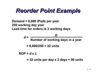
69. 12 - 70
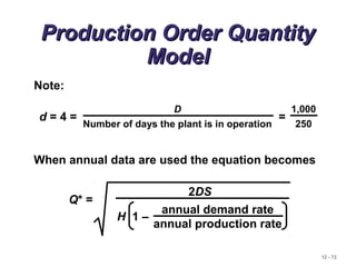
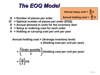
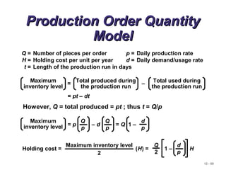
Production Order QuantityProduction Order Quantity
ModelModel
Q = Number of pieces per order p = Daily production rate
H = Holding cost per unit per year d = Daily demand/usage rate
D = Annual demand
Q2
=
2DS
H[1 - (d/p)]
Q* =
2DS
H[1 - (d/p)]p
Setup cost = (D/Q)S
Holding cost = HQ[1 - (d/p)]
1
2
(D/Q)S = HQ[1 - (d/p)]
1
2

70. 12 - 71
Production Order QuantityProduction Order Quantity
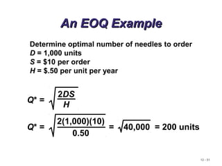
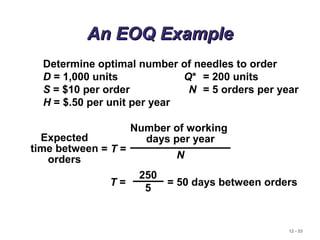
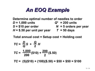
ExampleExample
D = 1,000 units p = 8 units per day
S = $10 d = 4 units per day
H = $0.50 per unit per year
Q* =
2DS
H[1 - (d/p)]
= 282.8 or 283 hubcaps
Q* = = 80,000
2(1,000)(10)
0.50[1 - (4/8)]

71. 12 - 72
Production Order QuantityProduction Order Quantity
ModelModel
When annual data are used the equation becomes
Q* =
2DS
annual demand rate
annual production rate
H 1 –
Note:
d = 4 = =
D
Number of days the plant is in operation
1,000
250

72. 12 - 73
Quantity Discount ModelsQuantity Discount Models
 Reduced prices are often available when
larger quantities are purchased
 Trade-off is between reduced product cost
and increased holding cost
Total cost = Setup cost + Holding cost + Product cost
TC = S + H + PD
D
Q
Q
2

73. 12 - 74
Quantity Discount ModelsQuantity Discount Models
Discount
Number Discount Quantity Discount (%)
Discount
Price (P)
1 0 to 999 no discount $5.00
2 1,000 to 1,999 4 $4.80
3 2,000 and over 5 $4.75
Table 12.2
A typical quantity discount schedule

74. 12 - 75
Quantity Discount ModelsQuantity Discount Models
1. For each discount, calculate Q*
2. If Q* for a discount doesn’t qualify,
choose the smallest possible order size
to get the discount
3. Compute the total cost for each Q* or
adjusted value from Step 2
4. Select the Q* that gives the lowest total
cost
Steps in analyzing a quantity discountSteps in analyzing a quantity discount

75. 12 - 76
Quantity Discount ModelsQuantity Discount Models
1,000 2,000
Totalcost$
0
Order quantity
Q* for discount 2 is below the allowable range at point a
and must be adjusted upward to 1,000 units at point b
a
b
1st price
break
2nd price
break
Total cost
curve for
discount 1
Total cost curve for discount 2
Total cost curve for discount 3
Figure 12.7

76. 12 - 77© 2011 Pearson Education, Inc. publishing as Prentice Hall
Price-Break Model Formula
CostHoldingAnnual
Cost)SetuporderDemand)(Or2(Annual
=
iC
2DS
=QOPT
Based on the same assumptions as the EOQ model,
the price-break model has a similar Qopt formula:
i = percentage of unit cost attributed to carrying inventory
C = cost per unit
Since “C” changes for each price-break, the formula
above will have to be used with each price-break cost
value

77. 12 - 78
Quantity Discount ExampleQuantity Discount Example
Calculate Q* for every discount
Q* =
2DS
IP
Q1* = = 700 cars/order
2(5,000)(49)
(.2)(5.00)
Q2* = = 714 cars/order
2(5,000)(49)
(.2)(4.80)
Q3* = = 718 cars/order
2(5,000)(49)
(.2)(4.75)

78. 12 - 79
Quantity Discount ExampleQuantity Discount Example
Calculate Q* for every discount
Q* =
2DS
IP
Q1* = = 700 cars/order
2(5,000)(49)
(.2)(5.00)
Q2* = = 714 cars/order
2(5,000)(49)
(.2)(4.80)
Q3* = = 718 cars/order
2(5,000)(49)
(.2)(4.75)
1,000 — adjusted
2,000 — adjusted

79. 12 - 80
Quantity Discount ExampleQuantity Discount Example
Discount
Number
Unit
Price
Order
Quantity
Annual
Product
Cost
Annual
Ordering
Cost
Annual
Holding
Cost Total
1 $5.00 700 $25,000 $350 $350 $25,700
2 $4.80 1,000 $24,000 $245 $480 $24,725
3 $4.75 2,000 $23.750 $122.50 $950 $24,822.50
Table 12.3
Choose the price and quantity that gives
the lowest total cost
Buy 1,000 units at $4.80 per unit

80. 12 - 81© 2011 Pearson Education, Inc. publishing as Prentice Hall
Price-Break Example Problem DataPrice-Break Example Problem Data
(Part 1)(Part 1)
A company has a chance to reduce their inventory ordering
costs by placing larger quantity orders using the price-break
order quantity schedule below. What should their optimal
order quantity be if this company purchases this single
inventory item with an e-mail ordering cost of $4, a carrying
cost rate of 2% of the inventory cost of the item, and an annual
demand of 10,000 units?
A company has a chance to reduce their inventory ordering
costs by placing larger quantity orders using the price-break
order quantity schedule below. What should their optimal
order quantity be if this company purchases this single
inventory item with an e-mail ordering cost of $4, a carrying
cost rate of 2% of the inventory cost of the item, and an annual
demand of 10,000 units?
Order Quantity(units) Price/unit($)
0 to 2,499 $1.20
2,500 to 3,999 1.00
4,000 or more .98

81. 12 - 82© 2011 Pearson Education, Inc. publishing as Prentice Hall
Price-Break Example Solution (Part 2)Price-Break Example Solution (Part 2)
units1,826=
0.02(1.20)
4)2(10,000)(
=
iC
2DS
=QOPT
Annual Demand (D)= 10,000 units
Cost to place an order (S)= $4
First, plug data into formula for each price-break value of “C”
units2,000=
0.02(1.00)
4)2(10,000)(
=
iC
2DS
=QOPT
units2,020=
0.02(0.98)
4)2(10,000)(
=
iC
2DS
=QOPT
Carrying cost % of total cost (i)= 2%
Cost per unit (C) = $1.20, $1.00, $0.98
Interval from 0 to 2499, the
Qopt value is feasible
Interval from 2500-3999, the
Qopt value is not feasible
Interval from 4000 & more, the
Qopt value is not feasible
Next, determine if the computed Qopt values are feasible or not

82. 12 - 84© 2011 Pearson Education, Inc. publishing as Prentice Hall
Price-Break Example Solution (Part 4)Price-Break Example Solution (Part 4)
iC
2
Q
+S
Q
D
+DC=TC
Next, we plug the true Qopt values into the total cost
annual cost function to determine the total cost under
each price-break
Next, we plug the true Qopt values into the total cost
annual cost function to determine the total cost under
each price-break
TC(0-2499)=(10000*1.20)+(10000/1826)*4+(1826/2)(0.02*1.20)
= $12,043.82
TC(2500-3999)= $10,041
TC(4000&more)= $9,949.20
TC(0-2499)=(10000*1.20)+(10000/1826)*4+(1826/2)(0.02*1.20)
= $12,043.82
TC(2500-3999)= $10,041
TC(4000&more)= $9,949.20
Finally, we select the least costly Qopt, which is this
problem occurs in the 4000 & more interval. In
summary, our optimal order quantity is 4000 units
Finally, we select the least costly Qopt, which is this
problem occurs in the 4000 & more interval. In
summary, our optimal order quantity is 4000 units