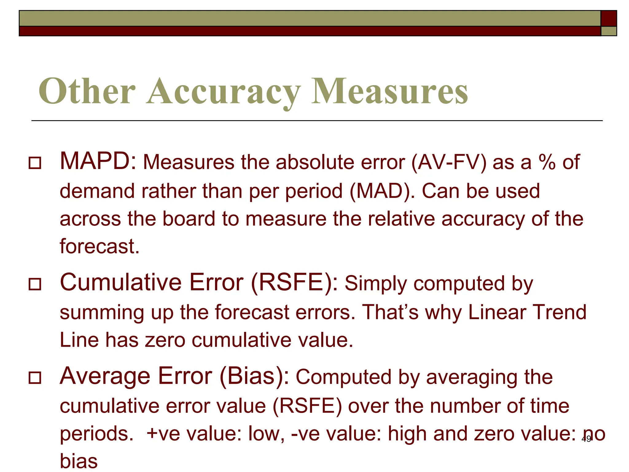
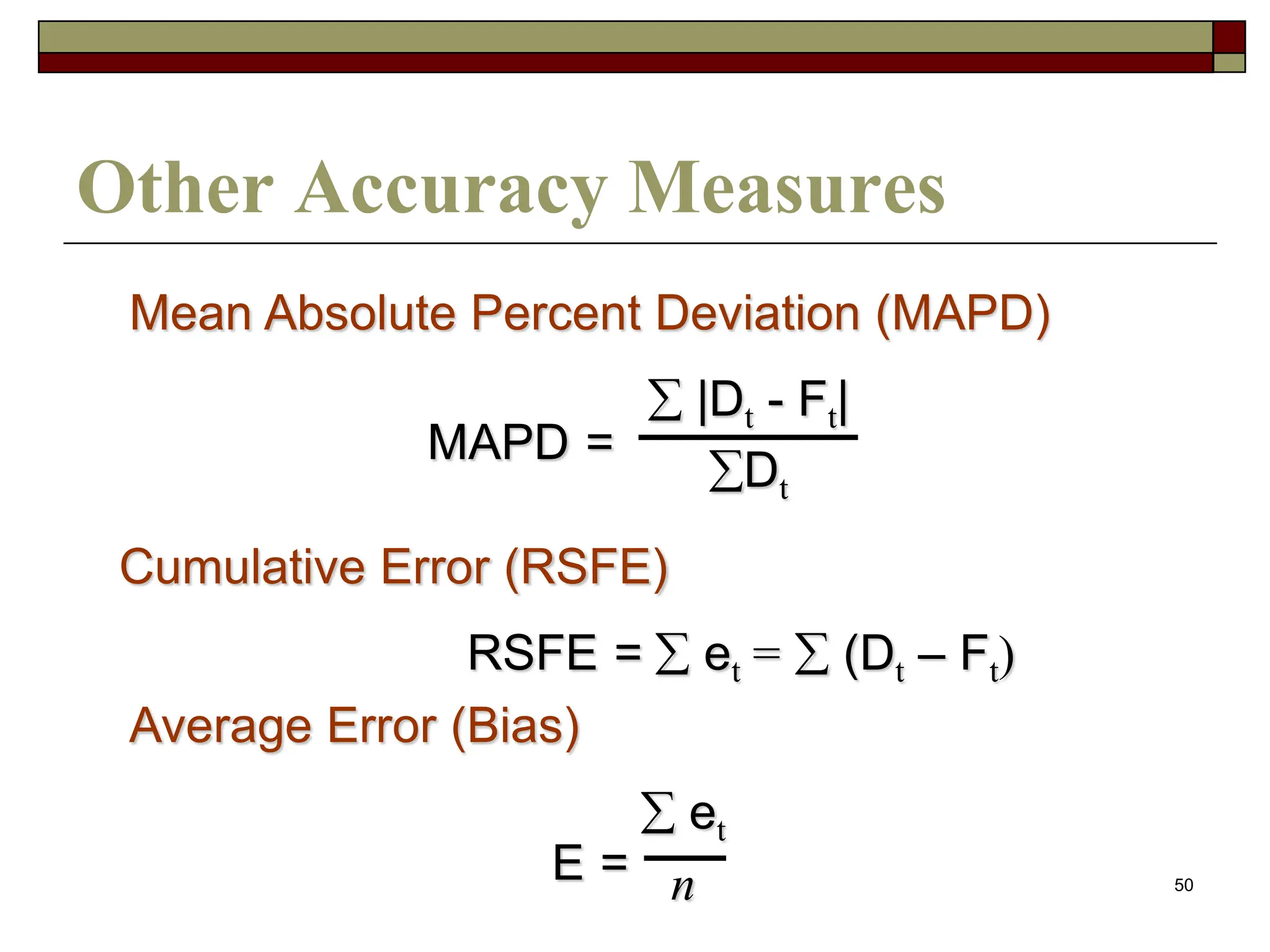
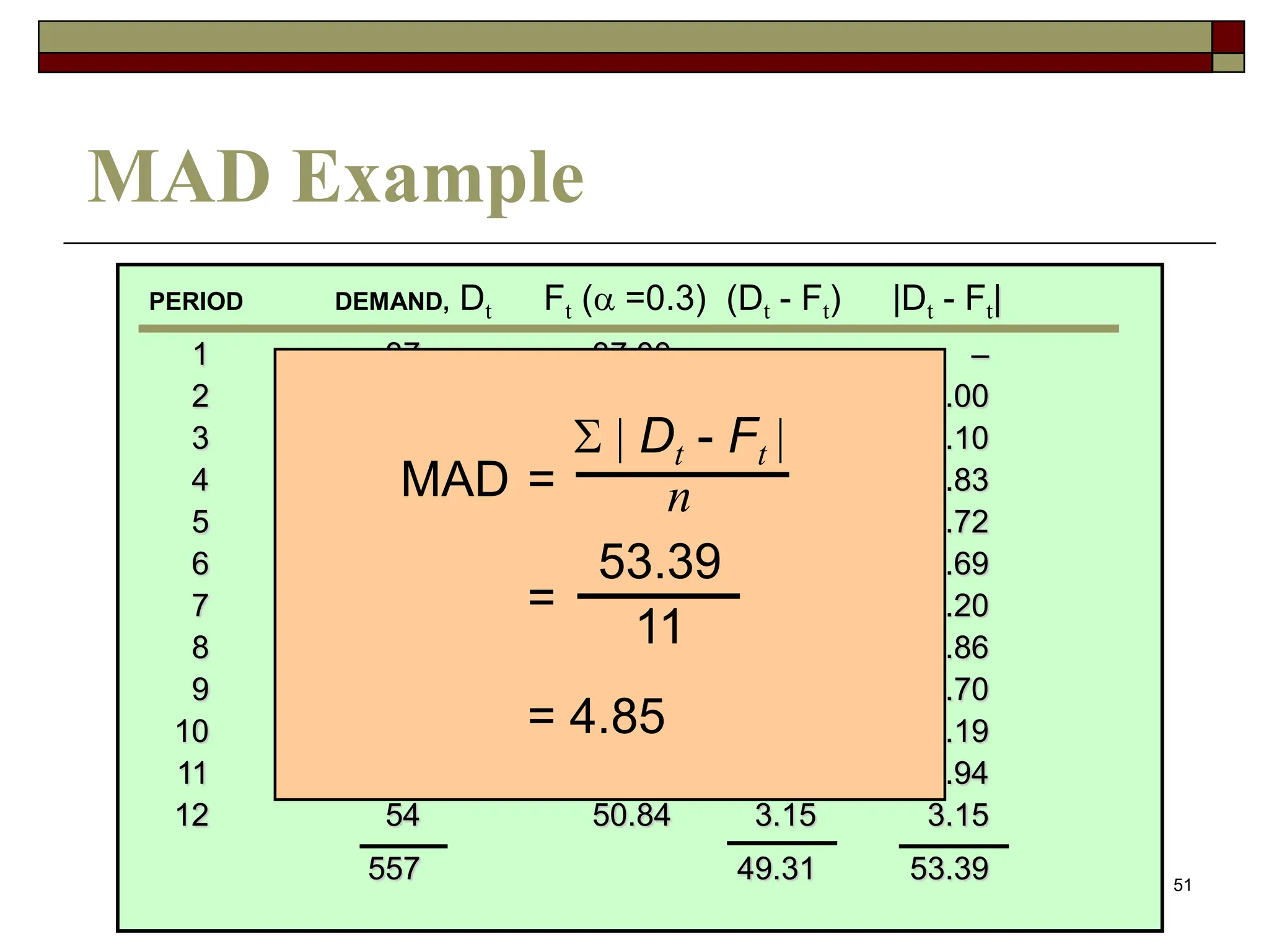
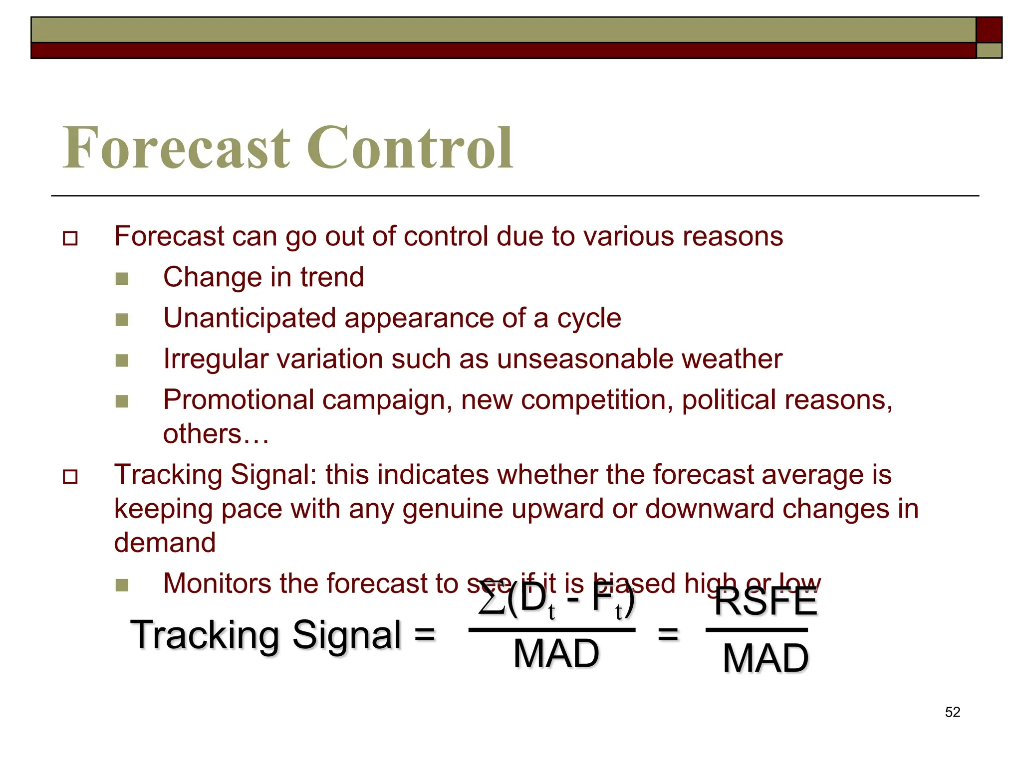
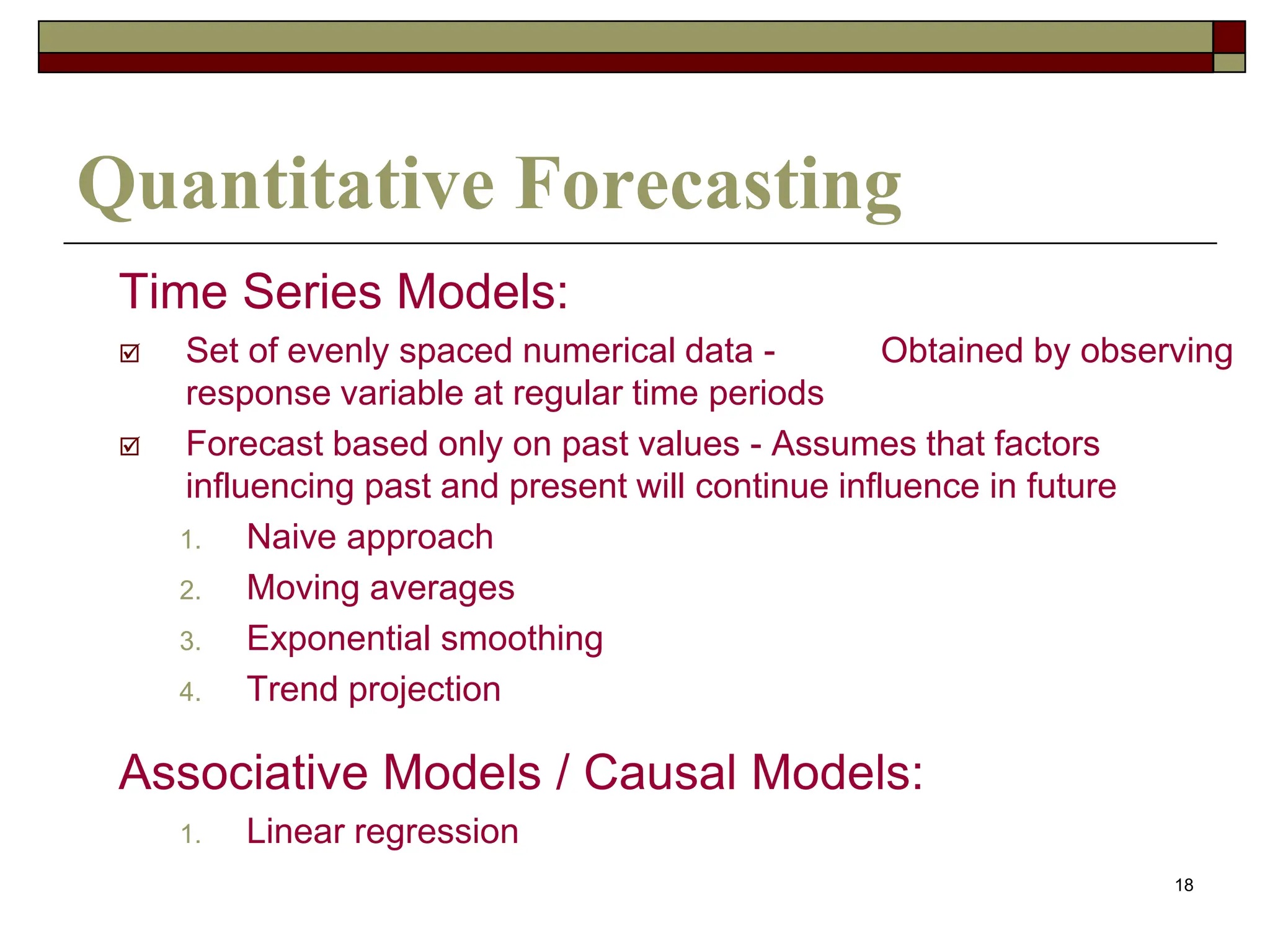
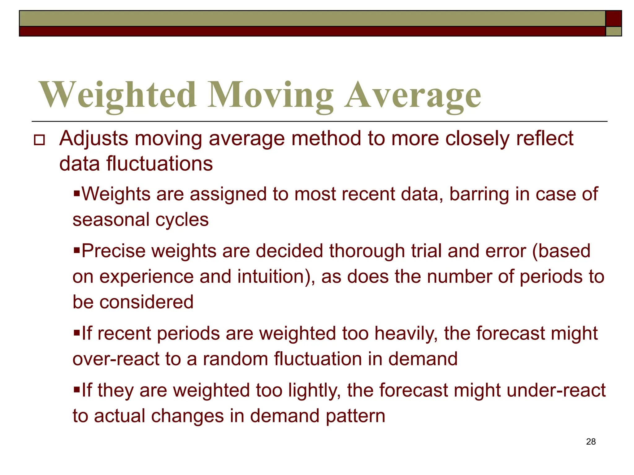
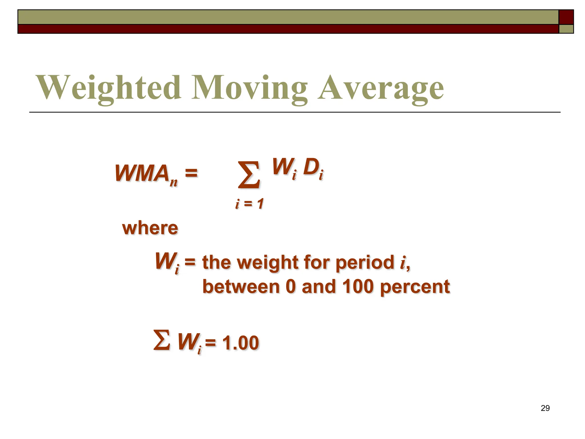
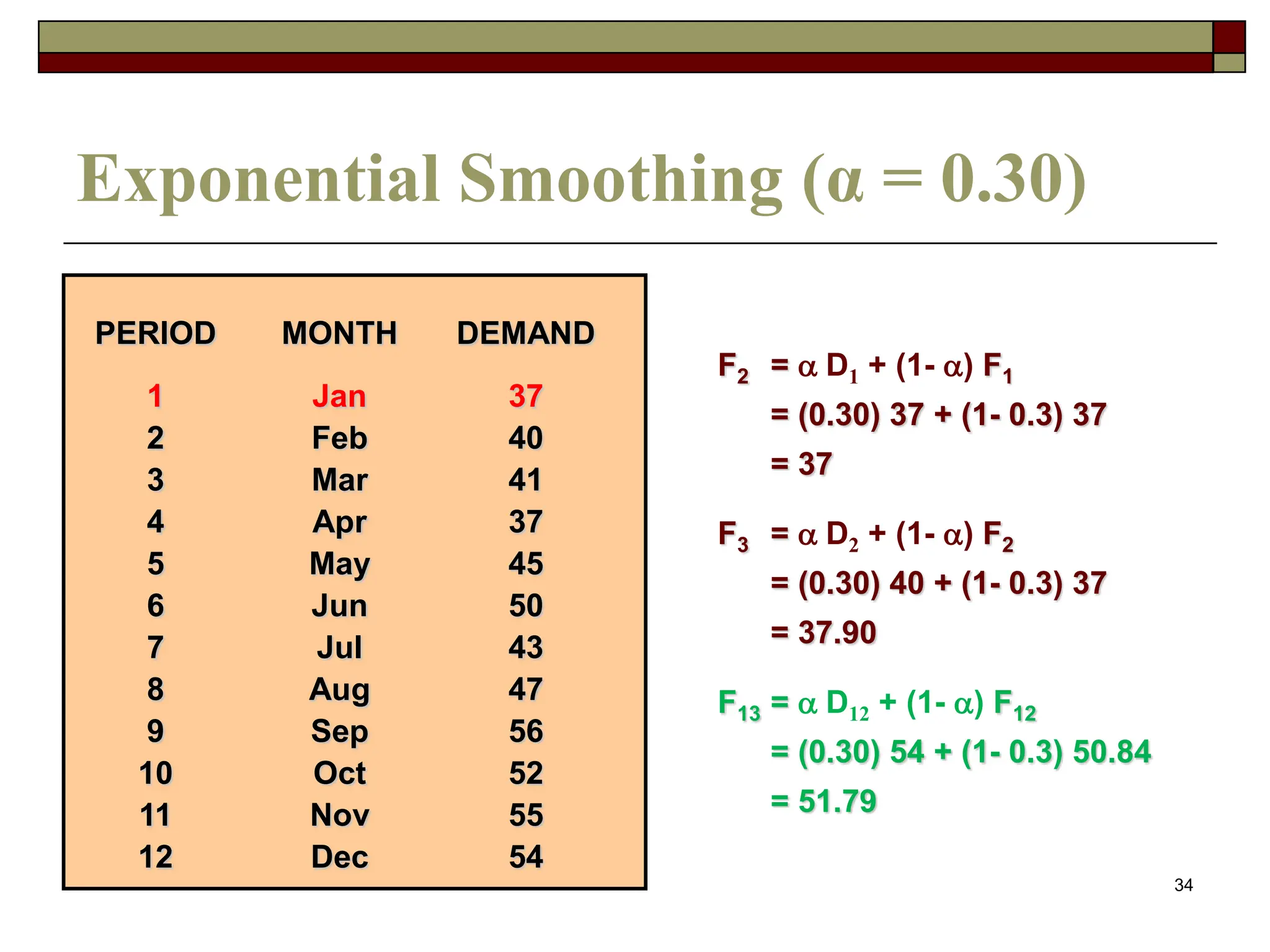
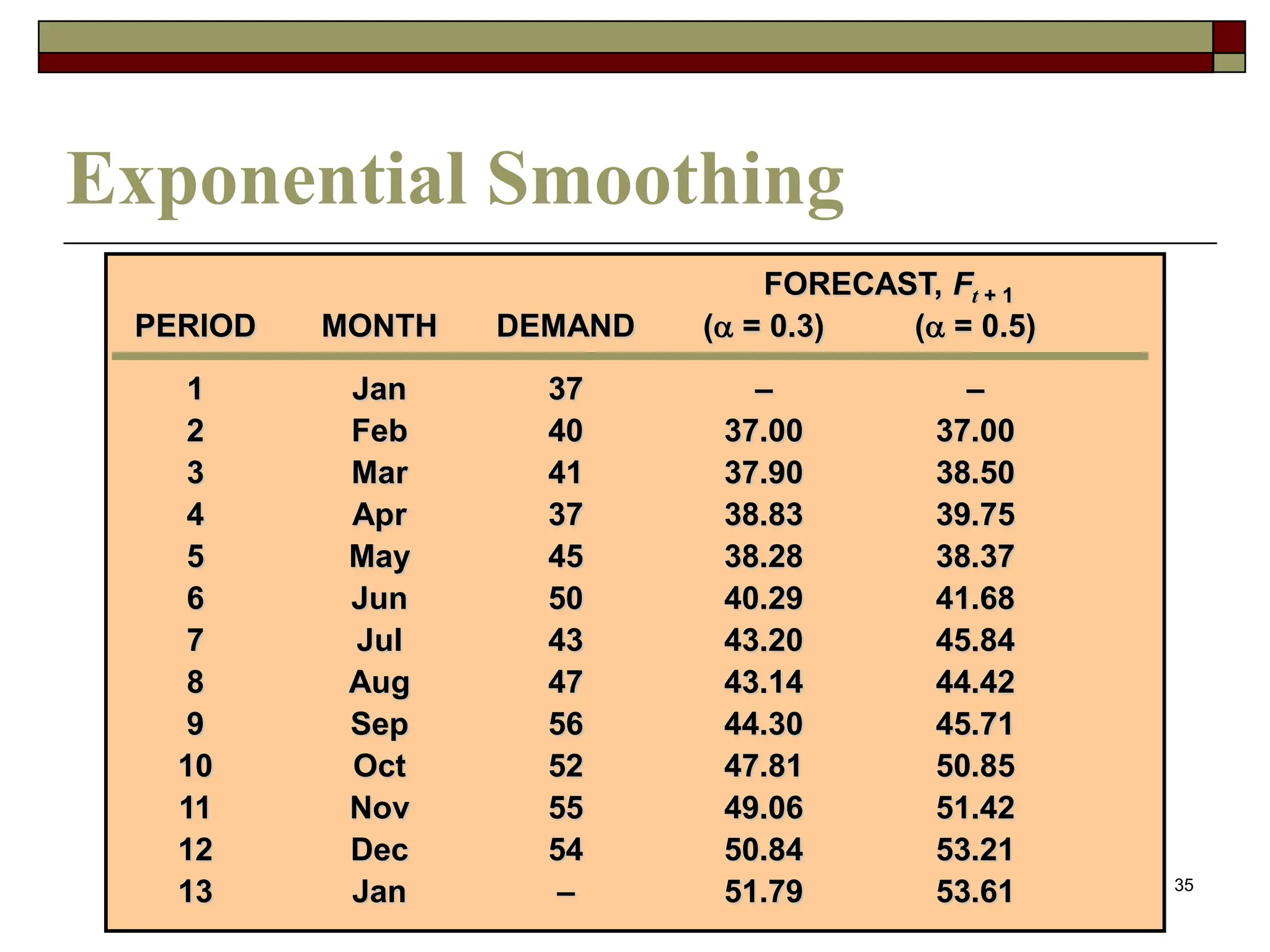
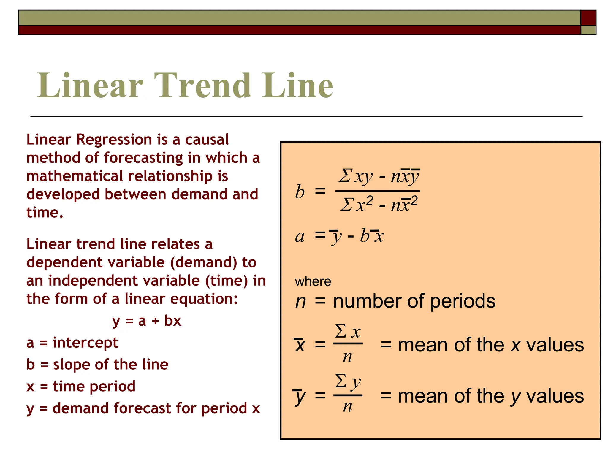
This document discusses various forecasting techniques. It begins by outlining qualitative and quantitative forecasting approaches. Several quantitative time series models are then described in detail, including naive methods, moving averages, exponential smoothing, and regression techniques. Specific examples are provided to illustrate how to calculate forecasts using simple and weighted moving averages, exponential smoothing with different alpha values, and linear regression with correlation and coefficient of determination. The document provides an overview of key forecasting concepts and quantitative methods.

1. 1
Forecasting

2. 2
Road Map
 Role of Forecasting
 Forecasting Approaches
 Qualitative forecasting
 Quantitative forecasting
 Time Series Models
 Regression Methods
 Forecast Accuracy
Focus Forecasting

3. 3
Forecasting
 Predicting the Future
 Vital for business
organization
 Underlying basis of
all business decisions
 Most techniques assume an
underlying stability in the
system
 Qualitative Forecasting Approach:
 Quantitative Forecasting
Approach:

4. 4

5. 5

6. 6

7. 7

8. 8

9. 9

10. 10

11. 11

12. 12

13. 13

14. 14

15. 15

16. 16

17. 17
Qualitative Methods
 Grass root method – going down to the lowest level of hierarchy
 Market research – data collection and hypothesis testing
 Jury of ‘executive opinion’ – source of internal qualitative forecast
 Historical analogy – history or past data of the item
 Panel consensus – free open exchange in between select few
 Delphi Method - Iterative group process
 3 types of participants
 Decision makers: Evaluate responses and make decisions
 Staff: Administering survey
 Respondents: People who can make valuable judgments

18. 18
Quantitative Forecasting
Time Series Models:
 Set of evenly spaced numerical data - Obtained by observing
response variable at regular time periods
 Forecast based only on past values - Assumes that factors
influencing past and present will continue influence in future
1. Naive approach
2. Moving averages
3. Exponential smoothing
4. Trend projection
Associative Models / Causal Models:
1. Linear regression

19. 19
Demand Behavior
 Trend
 Persistent, overall upward or downward pattern
 Changes due to population, technology, age, culture, etc.
 Cycle
 an up-&-down repetitive movement in demand over a length of span
 due to business cycle; political and economic factors
 Seasonal pattern
 is often weather / festival / event / specific period related
 oscillating in nature - usually occurs within a single year
 Random variations
 Erratic; unsystematic; short duration non-repeating
 unpredictable and have no “assignable causes”

20. 20
Time
(a) Trend
Time
(d) Trend with seasonal pattern
Time
(c) Seasonal pattern
Time
(b) Cycle
Demand
Demand
Demand
Demand
Random
movement
Forms of Forecast Movement

21. Demand
for
product
or
service
| | | |
1 2 3 4
Year
Average demand
over four years
Seasonal peaks
Trend component
Actual
demand
Random
variation
Components of Demand

22. 22
Moving Average
 Naive Forecast / Intuitive Forecast
 Demand of the current period is used as next period’s forecast
 Does not take into account historical behavior
 Reacts directly to the normal, random movements of the demand
 Cost effective and sometimes very efficient
 Simple Moving Average
 Uses several demand values during the recent past to forecast
 Tends to ‘smoothen’ or ‘dampen’, the random variations in single period
forecast
 Preferable for stable demand with no pronounced behavioral patterns
 Computed for specific number of periods depending on how the forecaster
desires to ‘smoothen’ the demand data
 The longer the moving average period, the smoother it will be.
 Alternatively, a shorter is more susceptible to simple random variations

23. 23
Naïve Approach
Jan 120
Feb 90
Mar 100
Apr 75
May 110
June 50
July 75
Aug 130
Sept 110
Oct 90
ORDERS
MONTH PER MONTH
-
120
90
100
75
110
50
75
130
110
90
Nov -
FORECAST

24. 24
Simple Moving Average
MAn =
n
i = 1
 Di
n
where
n = number of periods in
the moving average
Di = demand in period i

25. 25
3 Month Simple Moving Average
Jan 120
Feb 90
Mar 100
Apr 75
May 110
June 50
July 75
Aug 130
Sept 110
Oct 90
Nov -
ORDERS
MONTH PER MONTH
MA3 =
3
i = 1
 Di
3
=
120 + 90 + 100
3
= 103.3 orders for Apr.
–
–
–
103.3
88.3
95.0
78.3
78.3
85.0
105.0
110.0
MOVING
AVERAGE

26. 26
5 Month Simple Moving Average
Jan 120
Feb 90
Mar 100
Apr 75
May 110
June 50
July 75
Aug 130
Sept 110
Oct 90
Nov -
ORDERS
MONTH PER MONTH
MA5 =
5
i = 1
 Di
5
=
90 + 110 + 130+75+50
5
= 91 orders for Nov.
–
–
–
–
–
99.0
85.0
82.0
88.0
95.0
91.0
MOVING
AVERAGE

27. 27
Smoothing Effects
150 –
125 –
100 –
75 –
50 –
25 –
0 – | | | | | | | | | | |
Jan Feb Mar Apr May June July Aug Sept Oct Nov
Actual
Orders
Month
5-month
3-month

28. 28
Weighted Moving Average
 Adjusts moving average method to more closely reflect
data fluctuations
Weights are assigned to most recent data, barring in case of
seasonal cycles
Precise weights are decided thorough trial and error (based
on experience and intuition), as does the number of periods to
be considered
If recent periods are weighted too heavily, the forecast might
over-react to a random fluctuation in demand
If they are weighted too lightly, the forecast might under-react
to actual changes in demand pattern

29. 29
Weighted Moving Average
WMAn =
i = 1
 Wi Di
where
Wi = the weight for period i,
between 0 and 100 percent
 Wi = 1.00

30. 30
Weighted Moving Average
MONTH WEIGHT DATA
August 17% 130
September 33% 110
October 50% 90
WMA3 =
3
i = 1
 Wi Di
= (0.50) (90) + (0.33) (110) + (0.17) (130)
= 103.4 orders
November Forecast

31. 31
 Averaging method - weights most recent data more
strongly
 As the past becomes more distant, the imp. of data
diminishes
 So very useful and preferable method, if recent changes
are significant and unpredictable
 Widely used, most popular because its an accurate
method
 Requires minimal data:
forecast for the current period,
actual demand for the current period and
a weighing factor OR smoothing constant.
Exponential Smoothing

32. 32
Ft+1 =  *Dt + (1 - ) * Ft
where:
Ft + 1 =forecast for next period
Dt = actual demand for present period
Ft = previously determined forecast for present
period
 = weighting factor, smoothing constant –
determines the level of smoothing
*Assume first forecast as Actual Demand…
Exponential Smoothing

33. 33
Effect of Smoothing Constant
0.0  1.0
reflects the weight given to the most recent demand data
If = 0.20, then Ft + 1 = 0.20 * Dt + 0.8 * Ft
If = 0, then Ft + 1 = Ft
Forecast does not even consider recent actual data
If = 1, then Ft + 1 = 1 * Dt + 0 * Ft = Dt
Forecast based only on most recent data, so this becomes
as good as naïve forecast

34. 34
F2 =  D1 + (1- ) F1
= (0.30) 37 + (1- 0.3) 37
= 37
F3 =  D2 + (1- ) F2
= (0.30) 40 + (1- 0.3) 37
= 37.90
F13 =  D12 + (1- ) F12
= (0.30) 54 + (1- 0.3) 50.84
= 51.79
Exponential Smoothing (α = 0.30)
PERIOD MONTH DEMAND
1 Jan 37
2 Feb 40
3 Mar 41
4 Apr 37
5 May 45
6 Jun 50
7 Jul 43
8 Aug 47
9 Sep 56
10 Oct 52
11 Nov 55
12 Dec 54

35. 35
FORECAST, Ft + 1
PERIOD MONTH DEMAND ( = 0.3) ( = 0.5)
1 Jan 37 – –
2 Feb 40 37.00 37.00
3 Mar 41 37.90 38.50
4 Apr 37 38.83 39.75
5 May 45 38.28 38.37
6 Jun 50 40.29 41.68
7 Jul 43 43.20 45.84
8 Aug 47 43.14 44.42
9 Sep 56 44.30 45.71
10 Oct 52 47.81 50.85
11 Nov 55 49.06 51.42
12 Dec 54 50.84 53.21
13 Jan – 51.79 53.61
Exponential Smoothing

36. 36
70 –
60 –
50 –
40 –
30 –
20 –
10 –
0 – | | | | | | | | | | | | |
1 2 3 4 5 6 7 8 9 10 11 12 13
Actual
Orders
Month
Exponential Smoothing
 = 0.50
 = 0.30

37. 37
Regression Methods
 Linear Regression
 Regression can be defined as functional relationship between
two or more correlated variables
 Regression is used for forecasting by establishing a
mathematical relationship between two or more variables
(demand and some other independent variable) in the form of
a linear equation
 It is used to predict one variable given the other
 Linear regression refers to the special class of regression
where the relationship between the variable forms a straight
line
 Good for long range forecasting and aggregate planning

38. 38
Linear Regression is a causal
method of forecasting in which a
mathematical relationship is
developed between demand and
time.
Linear trend line relates a
dependent variable (demand) to
an independent variable (time) in
the form of a linear equation:
y = a + bx
a = intercept
b = slope of the line
x = time period
y = demand forecast for period x
Linear Trend Line
b =
a = y - b x
where
n = number of periods
x = = mean of the x values
y = = mean of the y values
xy - nxy
x2 - nx2
x
n
y
n

39. 39
Least Squares Example
x (PERIOD) y (DEMAND) x y x2
1 37 37 1
2 40 80 4
3 41 123 9
4 37 148 16
5 45 225 25
6 50 300 36
7 43 301 49
8 47 376 64
9 56 504 81
10 52 520 100
11 55 605 121
12 54 648 144
78 557 3867 650

40. 40
x = = 6.5
y = = 46.42
b = = =1.72
a = y - bx
= 46.42 - (1.72)(6.5) = 35.2
3867 - (12)(6.5)(46.42)
650 - 12(6.5)2
xy - nxy
x2 - nx2
78
12
557
12
Least Squares Example

41. 41
Linear Trend Line y = 35.2 + 1.72x
Forecast for Period 13 y = 35.2 + 1.72(13) = 57.56 units
70 –
60 –
50 –
40 –
30 –
20 –
10 –
0 –
| | | | | | | | | | | | |
1 2 3 4 5 6 7 8 9 10 11 12 13
Actual
Demand
Period
Linear trend line

42. 42
Linear Regression Example
x y
adv spend sales xy x2
4 36.3 145.2 16
6 40.1 240.6 36
6 41.2 247.2 36
8 53.0 424.0 64
6 44.0 264.0 36
7 45.6 319.2 49
5 39.0 195.0 25
7 47.5 332.5 49
49 346.7 2167.7 311

43. 43
Linear Regression Example (cont.)
x = = 6.125
y = = 43.36
b =
=
= 4.06
a = y - bx
= 43.36 - (4.06)(6.125)
= 18.46
49
8
346.9
8
xy - nxy
x2 - nx2
(2,167.7) - (8)(6.125)(43.36)
(311) - (8)(6.125)2

44. 44
| | | | | | | | | | |
0 1 2 3 4 5 6 7 8 9 10
60,000 –
50,000 –
40,000 –
30,000 –
20,000 –
10,000 –
Linear regression line,
y = 18.46 + 4.06x
Wins, x
Attendance,
y
Linear Regression Example (cont.)
y = 18.46 + 4.06x y = 18.46 + 4.06(7)
= 46.88, or 46,880
Regression equation Sales forecast for 7 lakhs of ad spend

45. 45
Correlation & Coefficient of Determination
 Correlation, r
 Correlation is a measure of the strength of the relationship
between independent and dependent variables
 degree of association between two variables (-1.00 to +1.00)
 nil/poor/average/strong, & positive/negative
 Coefficient of Determination, r2
 Percentage of variation in dependent variable resulting from
changes in the independent variable (0% to 100%)
 A measure of the amount of variation in the dependent variable
about its mean that is explained by the regression equation

46. 46
Computing Correlation
n xy -  x y
[n x2 - ( x)2] [n y2 - ( y)2]
r =
Coefficient of Determination
r2 = (0.947)2 = 0.897
r =
(8)(2,167.7) - (49)(346.9)
[(8)(311) - (49)2] [(8)(15,224.7) - (346.9)2]
r = 0.947

47. 47
Forecast Accuracy
 A forecast is never ever accurate
 Large degree of error mean
 Either the forecasting technique used is applied wrongly or is
not applicable in the case
 Wrong relationship among variables
 Or the ‘parameters’ used need to be adjusted for ‘trend’
 Forecast Error
 Difference between forecast and actual demand - Error
 MAD - Mean Absolute Deviation
 MAPD - Mean Absolute Percent Deviation or MAPE
 Cumulative Error - RSFE
 Average Error or Bias

48. 48
Mean Absolute Deviation (MAD)
MAD: The absolute average difference between the AD &
FD.
where,
t = period number
Dt = demand in period t
Ft = forecast for period t
n = total number of periods
 = absolute value
The smaller the value of MAD relative to the magnitude of
  Dt - Ft 
n
M A D =

49. 49
Other Accuracy Measures
 MAPD: Measures the absolute error (AV-FV) as a % of
demand rather than per period (MAD). Can be used
across the board to measure the relative accuracy of the
forecast.
 Cumulative Error (RSFE): Simply computed by
summing up the forecast errors. That’s why Linear Trend
Line has zero cumulative value.
 Average Error (Bias): Computed by averaging the
cumulative error value (RSFE) over the number of time
periods. +ve value: low, -ve value: high and zero value: no
bias

50. 50
Other Accuracy Measures
Mean Absolute Percent Deviation (MAPD)
MAPD =
 |Dt - Ft|
Dt
Cumulative Error (RSFE)
RSFE =  et =  (Dt – Ft)
Average Error (Bias)
E =
 et
n

51. 51
MAD Example
1 37 37.00 – –
2 40 37.00 3.00 3.00
3 41 37.90 3.10 3.10
4 37 38.83 -1.83 1.83
5 45 38.28 6.72 6.72
6 50 40.29 9.69 9.69
7 43 43.20 -0.20 0.20
8 47 43.14 3.86 3.86
9 56 44.30 11.70 11.70
10 52 47.81 4.19 4.19
11 55 49.06 5.94 5.94
12 54 50.84 3.15 3.15
557 49.31 53.39
PERIOD DEMAND, Dt Ft ( =0.3) (Dt - Ft) |Dt - Ft|
  Dt - Ft 
n
MAD =
=
= 4.85
53.39
11

52. 52
Forecast Control
 Forecast can go out of control due to various reasons
 Change in trend
 Unanticipated appearance of a cycle
 Irregular variation such as unseasonable weather
 Promotional campaign, new competition, political reasons,
others…
 Tracking Signal: this indicates whether the forecast average is
keeping pace with any genuine upward or downward changes in
demand
 Monitors the forecast to see if it is biased high or low
Tracking Signal = =
(Dt - Ft)
MAD
RSFE
MAD

53. 53
Tracking Signal Values
37 - – – - -
40 37.00 3.00 3.00 3.00 3.00
41 37.90 3.10 6.10 6.10 3.05
37 38.83 -1.83 4.27 7.93 2.64
45 38.28 6.72 10.99 14.65 3.66
50 40.29 9.69 20.68 24.34 4.87
43 43.20 -0.20 20.48 24.54 4.09
47 43.14 3.86 24.34 28.40 4.06
56 44.30 11.70 36.04 40.10 5.01
52 47.81 4.19 40.23 44.29 4.92
55 49.06 5.94 46.17 50.23 5.02
54 50.84 3.15 49.32 53.38 4.85
DEMAND FORECAST, ERROR RSEF = +ve CE
Dt Ft Dt - Ft (Dt - Ft)  Dt - Ft  MAD
TS3 = = 2.00
6.10
3.05
Tracking signal for period 3
1.00
2.00
1.62
3.00
4.25
5.01
6.00
7.19
8.18
9.20
10.17
TRACKING
SIGNAL

54. 54
Tracking Signal Plot
3 –
2 –
1 –
0 –
-1 –
-2 –
-3 –
| | | | | | | | | | | | |
0 1 2 3 4 5 6 7 8 9 10 11 12
Tracking
signal
(MAD)
Period
Exponential smoothing ( = 0.30)
Linear trend line

55. 55
Example
Example

56. 56
Example

57. 57
Example

58. 58
Seasonal Adjustments
 Repetitive increase / decrease in demand
 Seasonal patterns can also occur on a periodic basis
 Use seasonal factor to adjust forecast
 A seasonal factor is a numeric value that is multiplied
by the normal forecast to get a seasonally adjusted
forecast
 A seasonal factor range from 0 to 1, it is in effect, the
portion of annual demand assigned to each season
 Thus SF when multiplied to annual forecasted demand
yield seasonally adjusted forecasts for each season
Seasonal Factor =
Si =
Di
D

59. 59
Seasonal Adjustment (cont.)
2002 12.6 8.6 6.3 17.5 45.0
2003 14.1 10.3 7.5 18.2 50.1
2004 15.3 10.6 8.1 19.6 53.6
Total 42.0 29.5 21.9 55.3 148.7
DEMAND (1000’S PER QUARTER)
YEAR I II III IV Total
SI = = = 0.28
D1
D
42.0
148.7
SII = = = 0.20
D2
D
29.5
148.7
SIV = = = 0.37
D4
D
55.3
148.7
SIII = = = 0.15
D3
D
21.9
148.7

60. Seasonal Adjustment (cont.)
 X Y X*X X*Y
 1 45.0 1 45.00
 2 50.1 4 100.20
 3 53.6 9 160.80
 FIND MEAN OF X AND Y
 VALUE OF a AND b
60

61. 61
Seasonal Adjustment (cont.)
SFI = (SI) (F4) = (0.28)(58.17) = 16.28
SFII = (SII) (F4) = (0.20)(58.17) = 11.63
SFIII = (SIII) (F4) = (0.15)(58.17) = 8.73
SFIV = (SIV) (F4) = (0.37)(58.17) = 21.53
y = 40.97 + 4.30 x = 40.97 + 4.30(4) =
58.17
For 2005

62. 62
Forecasting Process
6. Check forecast
accuracy with one
or more measures
4. Select a forecast
model that seems
appropriate for data
5. Develop/compute
forecast for period
of historical data
8a. Forecast over
planning horizon
9. Adjust forecast
based on additional
qualitative info’ & insight
10. Monitor results
and measure
forecast accuracy
8b. Select new
forecast model or
adjust parameters
of existing model
7.
Is accuracy
of forecast
acceptable?
1. Identify the
purpose of forecast
3. Plot data and
identify patterns
2. Collect historical
data
No
Yes