The document discusses the JPEG image compression standard. It describes the basic JPEG compression pipeline which involves encoding, decoding, colour space transform, discrete cosine transform (DCT), quantization, zigzag scan, differential pulse code modulation (DPCM) on the DC component, run length encoding (RLE) on the AC components, and entropy coding using Huffman or arithmetic coding. It provides details on quantization methods, quantization tables, zigzag scan, DPCM, RLE, and Huffman coding used in JPEG to achieve maximal compression of images.

1. 426
Back
Close
Compression: Images (JPEG)
What is JPEG?
• JPEG: Joint Photographic Expert Group — an international
standard since 1992.
• Works with colour and greyscale images
• Up to 24 bit colour images (Unlike GIF)
• Target photographic quality images (Unlike GIF)
• Suitable for many applications e.g., satellite, medical, general
photography...

2. 427
Back
Close
Basic JPEG Compression Pipeline
JPEG compression involves the following:
• Encoding
• Decoding – Reverse the order for encoding

3. 428
Back
Close
Major Coding Algorithms in JPEG
The Major Steps in JPEG Coding involve:
• Colour Space Transform and subsampling (YIQ)
• DCT (Discrete Cosine Transformation)
• Quantisation
• Zigzag Scan
• DPCM on DC component
• RLE on AC Components
• Entropy Coding — Huffman or Arithmetic
We have met most of the algorithms already:
• JPEG exploits them in the compression pipeline to achieve
maximal overall compression.

4. 429
Back
Close
Quantisation
Why do we need to quantise:
• To throw out bits from DCT.
• Example: (101101)2 = 45 (6 bits).
Truncate to 4 bits: (1011)2 = 11.
Truncate to 3 bits: (101)2 = 5.
• Quantisation error is the main source of Lossy Compression.
• DCT itself is not Lossy
• How we throw away bits in Quantisation Step is Lossy

5. 430
Back
Close
Quantisation Methods
Uniform quantisation
• Divide by constant N and round result
(N = 4 or 8 in examples on previous page).
• Non powers-of-two gives fine control
(e.g., N = 6 loses 2.5 bits)

6. 431
Back
Close
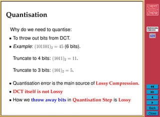
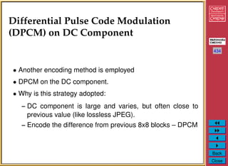
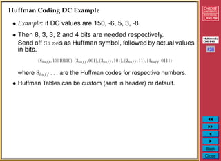
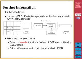
Quantisation Tables
• In JPEG, each F[u,v] is divided by a constant q(u,v).
• Table of q(u,v) is called quantisation table.
• Eye is most sensitive to low frequencies (upper left corner),
less sensitive to high frequencies (lower right corner)
• JPEG Standard defines 2 default quantisation tables, one for
luminance (below), one for chrominance. E.g Table below
----------------------------------
16 11 10 16 24 40 51 61
12 12 14 19 26 58 60 55
14 13 16 24 40 57 69 56
14 17 22 29 51 87 80 62
18 22 37 56 68 109 103 77
24 35 55 64 81 104 113 92
49 64 78 87 103 121 120 101
72 92 95 98 112 100 103 99
----------------------------------

7. 432
Back
Close
Quantization Tables (Cont)
• Q: How would changing the numbers affect the picture
E.g., if we doubled them all?
Quality factor in most implementations is the scaling factor for
default quantization tables.
• Custom quantization tables can be put in image/scan header.
JPEG Quantisation Example
• JPEG Quantisation Example (Java Applet)

8. 433
Back
Close
Zig-zag Scan
What is the purpose of the Zig-zag Scan:
• To group low frequency coefficients in top of vector.
• Maps 8 x 8 to a 1 x 64 vector

9. 434
Back
Close
Differential Pulse Code Modulation
(DPCM) on DC Component
• Another encoding method is employed
• DPCM on the DC component.
• Why is this strategy adopted:
– DC component is large and varies, but often close to
previous value (like lossless JPEG).
– Encode the difference from previous 8x8 blocks – DPCM

10. 435
Back
Close
Run Length Encode (RLE) on AC
Components
Yet another simple compression technique is applied to the
AC component:
• 1x63 vector (AC) has lots of zeros in it
• Encode as (skip, value) pairs, where skip is the number of
zeros and value is the next non-zero component.
• Send (0,0) as end-of-block sentinel value.

11. 436
Back
Close
Huffman (Entropy) Coding
DC and AC components finally need to be represented by a
smaller number of bits
(Arithmetic coding also supported in place of Huffman coding):
• (Variant of) Huffman coding: Each DPCM-coded DC
coefficient is represented by a pair of symbols :
(Size, Amplitude)
where Size indicates number of bits needed to represent
coefficient and
Amplitude contains actual bits.
• Size only Huffman coded in JPEG:
– Size does not change too much, generally smaller Sizes
occur frequently (= low entropy so is suitable for coding,
– Amplitude can change widely so coding no real benefit

12. 437
Back
Close
Huffman (Entropy) Coding (Cont)
• Example Size category for possible Amplitudes:
-------------------------------------------------
Size Typical Huffman Code for Size Amplitude
0 00 0
1 010 -1,1
2 011 -3,-2,2,3
3 100 -7..-4,4..7
4 101 -15..-8,8..15
. . .
. . .
--------------------------------------------------
• Use ones complement scheme for negative values: i.e 10 is
binary for 2 and 01 for -2 (bitwise inverse). Similarly, 00 for
-3 and 11 for 3.

13. 438
Back
Close
Huffman Coding DC Example
• Example: if DC values are 150, -6, 5, 3, -8
• Then 8, 3, 3, 2 and 4 bits are needed respectively.
Send off Sizes as Huffman symbol, followed by actual values
in bits.
(8huff , 10010110), (3huff , 001), (3huff , 101), (2huff , 11), (4huff , 0111)
where 8huff . . . are the Huffman codes for respective numbers.
• Huffman Tables can be custom (sent in header) or default.

14. 439
Back
Close
Huffman Coding on AC Component
AC coefficient are run-length encoded (RLE)
• RLE pairs (Runlength, Value) are Huffman coded as with
DC only on Value.
• So we get a triple: (Runlength, Size, Amplitude)
• However, Runlength, Size allocated 4-bits each and put
into a single byte with is then Huffman coded.
Again , Amplitude is not coded.
• So only two symbols transmitted per RLE coefficient:
(RLESIZEbytehuff, Amplitude)

15. 440
Back
Close
Example JPEG Compression

16. 441
Back
Close
Another Enumerated Example

17. 442
Back
Close
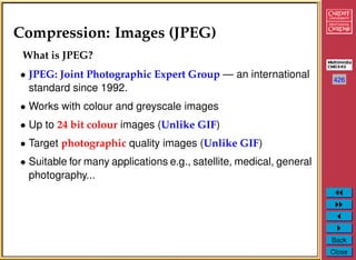
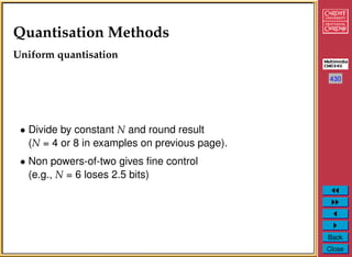
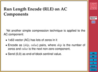
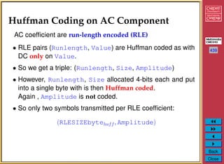
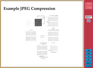
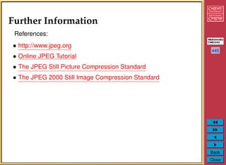
JPEG Example MATLAB Code
The JPEG algorithm may be summarised as follows,
im2jpeg.m (Encoder) jpeg2im.m (Decoder)
mat2huff.m (Huffman coder)
m = [16 11 10 16 24 40 51 61 % JPEG normalizing array
12 12 14 19 26 58 60 55 % and zig-zag reordering
14 13 16 24 40 57 69 56 % pattern.
14 17 22 29 51 87 80 62
18 22 37 56 68 109 103 77
24 35 55 64 81 104 113 92
49 64 78 87 103 121 120 101
72 92 95 98 112 100 103 99] * quality;
order = [1 9 2 3 10 17 25 18 11 4 5 12 19 26 33 ...
41 34 27 20 13 6 7 14 21 28 35 42 49 57 50 ...
43 36 29 22 15 8 16 23 30 37 44 51 58 59 52 ...
45 38 31 24 32 39 46 53 60 61 54 47 40 48 55 ...
62 63 56 64];
[xm, xn] = size(x); % Get input size.
x = double(x) - 128; % Level shift input
t = dctmtx(8); % Compute 8 x 8 DCT matrix
% Compute DCTs of 8x8 blocks and quantize the coefficients.
y = blkproc(x, [8 8], ’P1 * x * P2’, t, t’);
y = blkproc(y, [8 8], ’round(x ./ P1)’, m);

18. 443
Back
Close
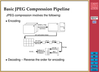
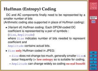
y = im2col(y, [8 8], ’distinct’); % Break 8x8 blocks into columns
xb = size(y, 2); % Get number of blocks
y = y(order, :); % Reorder column elements
eob = max(y(:)) + 1; % Create end-of-block symbol
r = zeros(numel(y) + size(y, 2), 1);
count = 0;
for j = 1:xb % Process 1 block (col) at a time
i = max(find(y(:, j))); % Find last non-zero element
if isempty(i) % No nonzero block values
i = 0;
end
p = count + 1;
q = p + i;
r(p:q) = [y(1:i, j); eob]; % Truncate trailing 0’s, add EOB,
count = count + i + 1; % and add to output vector
end
r((count + 1):end) = []; % Delete unusued portion of r
y = struct;
y.size = uint16([xm xn]);
y.numblocks = uint16(xb);
y.quality = uint16(quality * 100);
y.huffman = mat2huff(r);

19. 444
Back
Close
Further Information
Further standards:
• Lossless JPEG: Predictive approach for lossless compression
(why?), not widely used
• JPEG 2000: ISO/IEC 15444
– Based on wavelet transform, instead of DCT, no 8 × 8 blocks,
less artefacts
– Often better compression ratio, compared with JPEG

20. 445
Back
Close
Further Information
References:
• http://www.jpeg.org
• Online JPEG Tutorial
• The JPEG Still Picture Compression Standard
• The JPEG 2000 Still Image Compression Standard