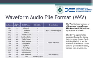
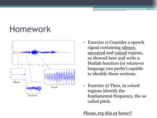
The document provides an introduction to audio signal processing and related topics. It discusses analog and digital audio signals, the waveform audio file format (WAV) specification including its header structure, and tools for audio processing like FFmpeg and MATLAB. Example code is given to read header metadata and audio samples from a WAV file in C++. While useful for understanding audio formats and processing, the solution contains an error and FFmpeg is noted as a better library for audio tasks.
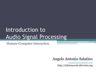
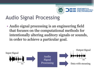
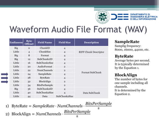
![Solution
typedef struct header_file
{
char chunk_id[4];
int chunk_size;
char format[4];
char subchunk1_id[4];
int subchunk1_size;
short int audio_format;
short int num_channels;
int sample_rate;
int byte_rate;
short int block_align;
short int bits_per_sample;
char subchunk2_id[4];
int subchunk2_size;
} header;
/************** Inside Main() **************/
header* meta = new header;
ifstream infile;
infile.exceptions (ifstream::eofbit | ifstream::failbit | ifstream::badbit);
infile.open("foo.wav", ios::in|ios::binary);
infile.read ((char*)meta, sizeof(header));
cout << " Header size: "<<sizeof(*meta)<<" bytes" << endl;
cout << " Sample Rate "<< meta->sample_rate <<" Hz" << endl;
cout << " Bits per samples: " << meta->bits_per_sample << " bit" <<endl;
cout << " Number of channels: " << meta->num_channels << endl;
long numOfSample = (meta->subchunk2_size/meta->num_channels)/(meta->bits_per_sample/8);
cout << " Number of samples: " << numOfSample << endl;
However, this solution contains an error. Can you spot it?](https://image.slidesharecdn.com/lectureonaudio-141030111326-conversion-gate01/85/Introductory-Lecture-to-Audio-Signal-Processing-16-320.jpg)
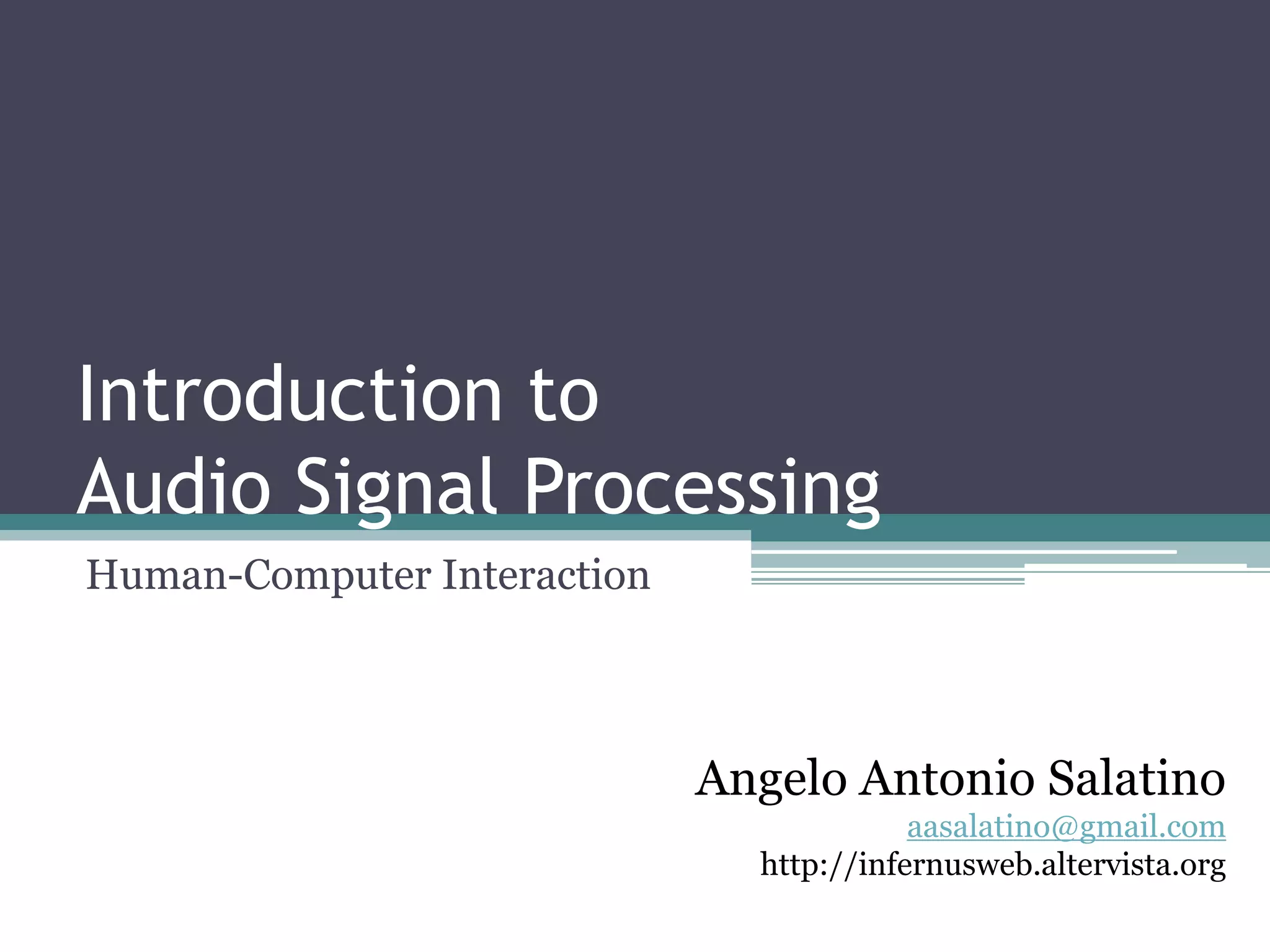
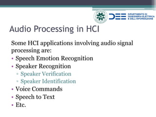
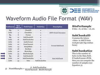
![What about reading samples?
short int* pU = NULL;
unsigned char* pC = NULL;
gWavDataIn = new double*[meta->num_channels]; //data structure storing the samples
for (int i = 0; i < meta->num_channels; i++) gWavDataIn[i] = new double[numOfSample];
wBuffer = new char[meta->subchunk2_size]; //data structure storing the bytes
/* data conversion: from byte to samples */
if(meta->bits_per_sample == 16)
{
pU = (short*) wBuffer;
for( int i = 0; i < numOfSample; i++)
for (int j = 0; j < meta->num_channels; j++)
gWavDataIn[j][i] = (double) (pU[i]);
}
else if(meta->bits_per_sample == 8)
{
pC = (unsigned char*) wBuffer;
for( int i = 0; i < numOfSample; i++)
for (int j = 0; j < meta->num_channels; j++)
gWavDataIn[j][i] = (double) (pC[i]);
}
else
{
printERR("Unhandled case");
}
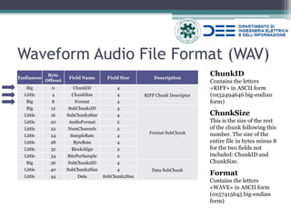
This solution is available at: https://github.com/angelosalatino/AudioSignalProcessing](https://image.slidesharecdn.com/lectureonaudio-141030111326-conversion-gate01/85/Introductory-Lecture-to-Audio-Signal-Processing-17-320.jpg)
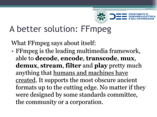
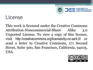
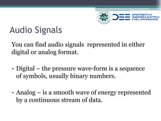
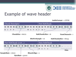
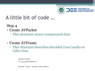
![A little bit of code …
Step 2
•Create AVStream
▫Stream structure; It contains: nb_frames, codec_context, duration and so on;
•Association between audio stream inside the context and the new one.
// Find the audio stream (some container files can have multiple streams in them) AVStream* audioStream = NULL; for (unsigned int i = 0; i < formatContext->nb_streams; ++i) if (formatContext->streams[i]->codec->codec_type == AVMEDIA_TYPE_AUDIO) { audioStream = formatContext->streams[i]; break; }](https://image.slidesharecdn.com/lectureonaudio-141030111326-conversion-gate01/85/Introductory-Lecture-to-Audio-Signal-Processing-21-320.jpg)
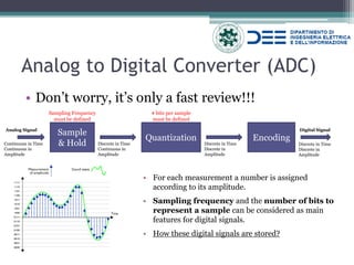
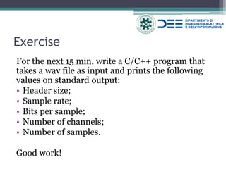
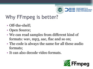
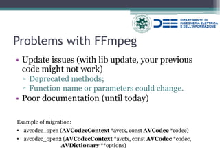
![A little bit of code …
Step 5
•Read packets
▫Packets are read from AVContextFormat
•Decode packets
▫Frame are decodec with CodecContext
// Read the packets in a loop
while (av_read_frame(formatContext, &packet) == 0)
{
…
avcodec_decode_audio4(codecContext, frame, &frameFinished, &packet);
…
src_data = frame->data[0];
}](https://image.slidesharecdn.com/lectureonaudio-141030111326-conversion-gate01/85/Introductory-Lecture-to-Audio-Signal-Processing-24-320.jpg)
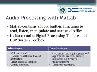
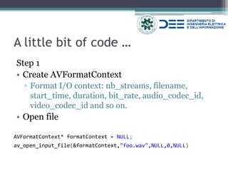
![Let’s code: Opening files
%% Reading file
% Section ID = 1
filename = './test.wav';
[data,fs] = wavread(filename); % reads only wav file
% data = sample collection, fs = sampling frequency
% or ---> [data,fs] = audioread(filename);
% write an audio file
audiowrite('./testCopy.wav',data,fs)
Recognized formats by audioread()](https://image.slidesharecdn.com/lectureonaudio-141030111326-conversion-gate01/85/Introductory-Lecture-to-Audio-Signal-Processing-27-320.jpg)
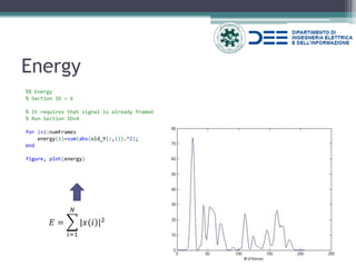
![Framing
%% Framing
% Section ID = 4
timeWindow = 0.04; % Frame length in term of seconds. Default: timeWindow = 40ms
timeStep = 0.01; % seconds between two frames. Default: timeStep = 10ms (in case of OVERLAPPING)
overlap = 1; % 1 in case of overlap, 0 no overlap
sampleForWindow = timeWindow * fs;
if overlap == 0;
Y = buffer(data,sampleForWindow);
else
sampleToJump = sampleForWindow - timeStep * fs;
Y = buffer(data,sampleForWindow,ceil(sampleToJump));
end
[m,n]=size(Y); % m corresponds to sampleForWindow
numFrames = n;
disp(sprintf('Number of Frames: %d',numFrames));
푠(푡)=푥(푡)⋅푟푒푐푡 푡−휏 #푠푎푚푝푙푒](https://image.slidesharecdn.com/lectureonaudio-141030111326-conversion-gate01/85/Introductory-Lecture-to-Audio-Signal-Processing-29-320.jpg)
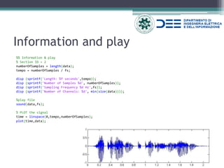
![Windowing
%% Windowing
% Section ID = 5
num_points = sampleForWindow;
% some windows USE help window
w_gauss = gausswin(num_points);
w_hamming = hamming(num_points);
w_hann = hann(num_points);
plot(1:num_points,[w_gauss,w_hamming, w_hann]); axis([1 num_points 0 2]);
legend('Gaussian','Hamming','Hann');
old_Y = Y;
for i=1:numFrames
Y(:,i)=Y(:,i).*w_hann;
end
%see the difference
index_to_plot = 88;
figure
plot (old_Y(:,index_to_plot))
hold on
plot (Y(:,index_to_plot), 'green')
hold off
clear num_points w_gauss w_hamming w_hann
푤퐺퐴푈푆푆(푛)=푒 − 12 푛−(푁−1)2 휎(푁−1)2 2,휎≤ 0.5
푤퐻퐴푀푀퐼푁퐺(푛)=0.54+0.46 cos2휋푛 푁−1
푤퐻퐴푁푁(푛)=0.5 1+cos2휋푛 푁−1](https://image.slidesharecdn.com/lectureonaudio-141030111326-conversion-gate01/85/Introductory-Lecture-to-Audio-Signal-Processing-30-320.jpg)
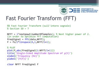
![Short Term Fourier Transform (STFT)
%% Short Term Fourier Transform
% Section ID = 8
% It requires that signal is already framed. Run Section ID=4
NFFT = 2^nextpow2(sampleForWindow);
STFT = ones(NFFT,numFrames);
for i=1:numFrames
STFT(:,i)=fft(Y(:,i),NFFT);
end
indexToPlot = 80; %frame index to plot
if indexToPlot < numFrames
f = fs/2*linspace(0,1,NFFT/2+1);
plot(f,2*abs(STFT(1:NFFT/2+1,indexToPlot))) % PLOT
title(sprintf('FFT del frame %d', indexToPlot));
xlabel('Frequency (Hz)')
ylabel(sprintf('|STFT_{%d}(f)|',indexToPlot))
else
disp('Unable to create plot');
End
% *********************************************
specgram(data,sampleForWindow,fs) % SPECTROGRAM
title('Spectrogram [dB]')](https://image.slidesharecdn.com/lectureonaudio-141030111326-conversion-gate01/85/Introductory-Lecture-to-Audio-Signal-Processing-33-320.jpg)
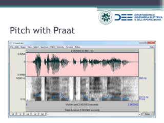


![Early Detection of Research Trends [thesis defence]](https://cdn.slidesharecdn.com/ss_thumbnails/thesisdefence2-191021145854-thumbnail.jpg?width=640&height=640&fit=bounds)


