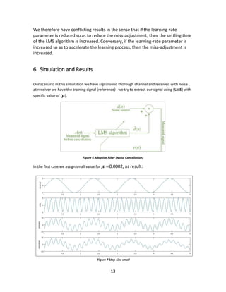
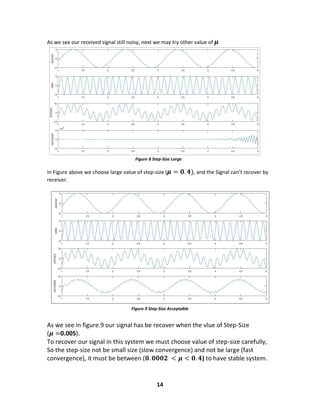
This document provides an overview of adaptive filtering techniques. It discusses digital filters and classifications such as linear/nonlinear and finite impulse response (FIR)/infinite impulse response (IIR). It then covers Wiener filters, including how they minimize mean square error. The method of steepest descent is presented as an approach to solve the Wiener-Hopf equations to find optimal filter weights. Finally, it discusses how the least mean squares (LMS) algorithm can be used for adaptive filtering by updating filter weights recursively in the direction that reduces mean square error.


![5
Response (FIR) filter.
In general, the formulation of an IIR Wiener filter results in a set of non-linear
equations, whereas the formulation of an FIR Wiener filter results in a set of
linear equations and has a closed-form solution e they are relatively simple to
compute, inherently stable and more practical. The main drawback of FIR filters
compared with IIR filters is that they may need a large number of coefficients to
approximate a desired response.
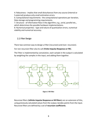
Figure 3 Wiener Filters
Where 𝑥( 𝑛) is input signal and 𝑤 are filter coefficients, respectively; that is
𝑥(𝑛) = [ 𝑥(𝑛)𝑥 … 𝑥(𝑛 − 𝑁 + 1)] 𝑇
(1)
𝑤 = [ 𝑤0 𝑤1 … . 𝑤 𝑁] 𝑇
(2)
And 𝑦(𝑘) is the output signal,
𝑦(𝑛) = ∑ 𝑤𝑖 𝑥(𝑛 − 𝑖)𝑁
𝑖=0
= 𝑤𝑜 𝑥(𝑛) + 𝑤1 𝑥(𝑛 − 1) + ⋯ + 𝑤 𝑁 𝑥(𝑛 − 𝑁)
𝑦(𝑛) = 𝑤 𝑇
𝑥(𝑛) (3)
𝑑(𝑛) Is the training or desired signal, and e(n) is error signal (different between the
Output signal 𝑦(𝑛) and desired signal 𝑑(𝑛)).
𝑒(𝑛) = 𝑑(𝑛) − 𝑦(𝑛) (4)](https://image.slidesharecdn.com/adaptivefilters-160111213909/85/Adaptive-filters-7-320.jpg)
![6
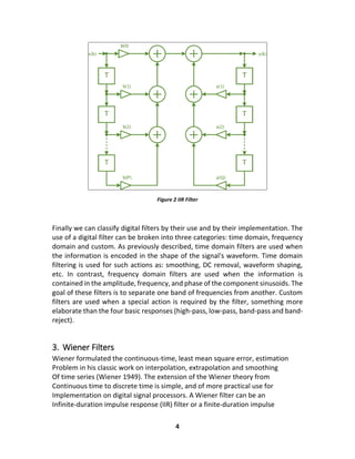
3.1.Error Measurements
Adaptation of the filter coefficients follows a minimization procedure of a
particular objective or cost function. This function is commonly defined as a norm
of the error signal e (n). The most commonly employed norms are the mean-
square error (MSE).
3.2.The Mean-Square Error (MSE).
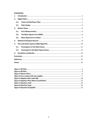
From Figure 3, we defined The MSE (cost function) as
𝜉(𝑛) = 𝐸[𝑒2(𝑛)] = 𝐸[| 𝑑(𝑛) − 𝑦(𝑛)|2]. (5)
From equation (3) we write the equation (5) as follow:
So,
𝜉(𝑛) = 𝐸[𝑒2(𝑛)] = 𝐸[| 𝑑(𝑛) − 𝑦(𝑛)|2]
𝜉(𝑛) = 𝐸[𝑒2(𝑛)] = 𝐸[| 𝑑(𝑛) − 𝑤 𝑇
𝑥(𝑛)|2]
𝜉(𝑛) = [𝑑2(𝑛) − 2𝑤 𝑇
𝐸[𝑑(𝑛)𝑥(𝑛)] + 𝑤 𝑇
𝐸[𝑥(𝑛)𝑤 𝑇
𝐸[𝑥(𝑛)𝑥 𝑇(𝑛)]𝑤
Where,
𝑅= 𝐸[𝑥(𝑛)𝑥 𝑇(𝑛)],
𝑝 = 𝐸[𝑑(𝑛)𝑥 𝑇(𝑛)].
𝜉(𝑛) = 𝑥 𝑑𝑑(0) − 2𝑝 + 2𝑅𝑤 (6)
Where R and p are the input-signal correlation matrix and the cross-correlation
vector between the reference signal and the input signal.
The gradient vector of the MSE function with respect to the adaptive filter
coefficient vector is given by
∇w ξ (n)= −2𝑝 + 2𝑅𝑤 (7)
That minimizes the MSE cost function, is obtained by equating the gradient
vector to zero. Assuming that R is non-singular, one gets that
∇ 𝑤 𝜉(𝑛) = 0](https://image.slidesharecdn.com/adaptivefilters-160111213909/85/Adaptive-filters-8-320.jpg)
![8
4. Method of Steepest Descent
To solve the Wiener-Hopf equations (Eq.7) for tap weights of the optimum spatial
filter, we basically need to compute the inverse of a p-by-p matrix made up of the
different values of the autocorrelation function. We may avoid the need for this
matrix inversion by using the method of steepest descent. Starting with an initial
guess for optimum weight 𝒘 𝒐, say 𝒘(𝟎), a recursive search method that may
require many iterations (steps) to converge to 𝒘 𝒐 is used.
The method of steepest descent is a general scheme that uses the following steps
to search for the minimum point of any convex function of a set of parameters:
1. Start with an initial guess of the parameters whose optimum values are to
be found for minimizing the function.
2. Find the gradient of the function with respect to these parameters at the
present point.
3. Update the parameters by taking a step in the opposite direction of the
gradient vector obtained in Step 2. This corresponds to a step in the direction
of steepest descent in the cost function at the present point. Furthermore,
the size of the step taken is chosen proportional to the size of the gradient
vector.
4. Repeat Steps 2 and 3 until no further significant change is observed in the
parameters.
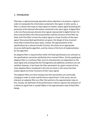
To implement this procedure in the case of the transversal filter shown in Figure
3, we recall (equation 7)
∇w ξ (n)= −2𝑝 + 2𝑅𝑤 (9)
Where ∇ is the gradient operator defined as the column vector,
∇ = [
𝜕
𝜕𝑤0
𝜕
𝜕𝑤1
…
𝜕
𝜕𝑤 𝑁−1
]
𝑇
(10)
According to the above procedure, if 𝑤(𝑛) is the tap-weight vector at the 𝑛 𝑡ℎ
iteration, the following recursive equation may be used to update 𝑤( 𝑛).
𝑤( 𝑛 + 1) = 𝑤( 𝑛) − 𝜇∇ 𝑘 𝜉 (11)
Where 𝜇 positive scalar is call Step-Size, and ∇ 𝑘 𝜉 denotes the gradient vector ∇ 𝑘 𝜉
evaluated at the point 𝑤 = 𝑤( 𝑘). Substituting (Eq.9) in (Eq. 11), we get
𝑤( 𝑛 + 1) = 𝑤( 𝑛) − 2𝜇(𝑅𝑤( 𝑛) − 𝑝) (12)](https://image.slidesharecdn.com/adaptivefilters-160111213909/85/Adaptive-filters-10-320.jpg)
![9
As we shall soon show, the convergence of 𝒘(𝒏) to the optimum solution
𝑤𝑜 and the speed at which this convergence takes place are dependent on the
size of the step-size parameter μ. A large step-size may result in divergence of
this recursive equation.
To see how the recursive update 𝑤(𝑘) converges toward𝑤𝑜, we rearrange Eq.
(12) as
𝑤( 𝑘 + 1) = (Ι − 2𝜇𝑹) 𝒘( 𝑘) + 2𝜇𝒑 (13)
Where 𝚰 is the N-by-N identify matrix. Next we subtract 𝑤𝑜form both side for Eq.
(13) and rearrange the result to obtain
𝑤( 𝑘 + 1) − 𝑤𝑜 = (Ι − 2𝜇𝑹)( 𝒘( 𝑘) − 𝒘 𝒐) (14)
Defining the 𝑐( 𝑘) as
𝑐( 𝑛) = 𝑤( 𝑛) − 𝑤𝑜
And 𝑅 = 𝑄Λ𝑄 𝑇
Where 𝚲 is a diagonal matrix consisting of the eigenvalues 𝜆0, 𝜆0, … 𝜆 𝑁−1 of R and
the columns of 𝑄 contain the corresponding orthonormal eigenvectors,
and Ι =𝑄𝑄 𝑇
, Substituting Eq.(14) we get
𝑐( 𝑛 + 1) = 𝑄(I − 2μΛ) 𝑄 𝑇
𝑣( 𝑘) (15)
Pre-multiplying Eq. (15) by 𝑄 𝑇
we have 𝑄 𝐻
𝑐( 𝑛 + 1) = (I − μΛ)𝑄 𝐻
𝑐(𝑛) (16)
Notation: 𝑣( 𝑛) = 𝑄 𝐻
𝑐(𝑛)
𝑣( 𝑛 + 1) = (I − μΛ) 𝑣( 𝑛), 𝑘 = 1,2, . . , 𝑁 (17)
Initial conditions: 𝑣(0) = 𝑄 𝐻
𝑐(0) = 𝑄 𝐻
[𝑤(0) − 𝑤𝑜]
𝑣 𝑘( 𝑛) = (1 − 𝜇𝜆 𝑚𝑎𝑥) 𝑛
𝑣 𝑘(0), 𝑘 = 1,2, … . , 𝑁
Convergence (stability):
When n=0, 0 < 𝜇 <
2
𝜆 𝑚𝑎𝑥
Stability condition
𝜆 𝑚𝑎𝑥 = max{𝜆1, 𝜆2, … , 𝜆 𝑁}
𝜆 𝑚𝑎𝑥 Is the maximum of the eigenvalues𝜆0 , 𝜆1, … . , 𝜆 𝑁−1. The left limit in refers to
the fact that the tap-weight correction must be in the opposite direction of the
gradient vector. The right limit is to ensure that all the scalar tap-weight
parameters in the recursive equations (17) decay exponentially as 𝑘 increases.](https://image.slidesharecdn.com/adaptivefilters-160111213909/85/Adaptive-filters-11-320.jpg)
![10
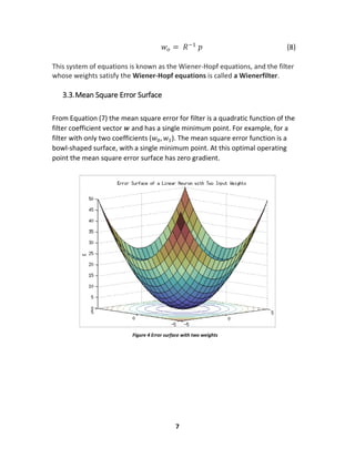
5. The Least Mean Squares (LMS) Algorithm
In any event, care has to be exercised in the selection of the learning-rate
parameter 𝝁 for the method of steepest descent to work. Also, a practical
limitation of the method of steepest descent is that it requires knowledge of the
spatial correlation functions 𝒓 𝒅𝒙( 𝒋, 𝒏)and 𝒓 𝒙𝒙(𝒋, 𝒏)now, when the filter operates
in an unknown environment, these correlation functions are not available, in
which case we are forced to use estimates in their place. The least-mean-square
algorithm results from a simple and yet effective method of providing for these
estimates.
The least-mean-square (LMS) algorithm is based on the use of instantaneous
estimates of the autocorrelation function 𝑹 and the cross-correlation function
𝒑.These estimates are deduced directly from the defining equations (18) and (19)
as follows:
𝑅= 𝐸[𝑥(𝑛)𝑥 𝑇(𝑛)] ⟹ 𝑅′
= 𝑥(𝑛)𝑥 𝑇(𝑛) (18)
𝑝 = 𝐸[𝑑(𝑛)𝑥 𝑇(𝑛)] ⇒ 𝑝′
= 𝑥(𝑛)𝑑(𝑛) (19)
Now call Eq. (12): 𝑤( 𝑛 + 1) = 𝑤( 𝑛) − 2𝜇( 𝑅𝑤( 𝑛) − 𝑝)
𝑤( 𝑛 + 1) = 𝑤( 𝑛) − 2𝜇[( 𝑥( 𝑛) 𝑥 𝑇( 𝑛) 𝑤( 𝑛) − 𝑥( 𝑛) 𝑑( 𝑛)]
𝑤( 𝑛 + 1) = 𝑤( 𝑛) − 2𝜇𝑥(𝑛)[( 𝑥( 𝑛) 𝑥 𝑇( 𝑛) 𝑤( 𝑛) − 𝑑( 𝑛)]
When 𝑒′
(𝑛) = ( 𝑥( 𝑛) 𝑥 𝑇( 𝑛) 𝑤( 𝑛) − 𝑑( 𝑛)
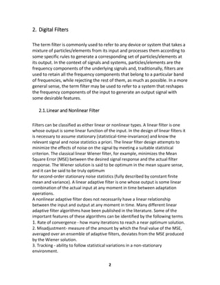
So, 𝑤( 𝑛 + 1) = 𝑤( 𝑛) − 2𝜇𝑥(𝑛)𝑒′
(𝑛) (20)
Equation (20) describe Least-Mean-Square (LMS) Algorithm.
Figure 5 Adaptive Filter with LMS](https://image.slidesharecdn.com/adaptivefilters-160111213909/85/Adaptive-filters-12-320.jpg)
![11
Summary of the LMS algorithm
Input: Tap-weight vector, 𝒘( 𝒏),
Input vector, 𝒙(𝒏).
and desired output, 𝒅(𝒏).
Output: Filter: output, 𝒚(𝒏)
Tap-weight vector update 𝒘( 𝒏 + 𝟏)
1. Filtering:
𝒚(𝒏) = 𝒘 𝑻
𝒙(𝒏)
2. Error Estimation:
𝒆(𝒏) = 𝒅(𝒏) − 𝒚(𝒏)
3. Tap-Weight Vector Adaptation:
𝒘( 𝒏 + 𝟏) = 𝒘( 𝒏) − 𝟐𝝁𝒙(𝒏)𝒆′
(𝒏)
Where 𝑥( 𝑛) = [ 𝑥( 𝑛) 𝑥… 𝑥( 𝑛 − 𝑁 + 1)] 𝑇 . Substituting this result in Eq. (11),
we get
𝑤( 𝑛 + 1) = 𝑤( 𝑛) + 2𝜇𝑒( 𝑛) 𝑥( 𝑛) (21)
This is referred to as the LMS recursion it suggests a simple procedure for
recursive adaptation of the filter coefficients after arrival of every new input
sample 𝑥( 𝑛) and its corresponding desired output sample, 𝑑( 𝑛) Equations (3),
(4), and (21), in this order, specify the three steps required to complete each
iteration of the LMS algorithm. Equation (3) is referred to as filtering. It is
performed to obtain the filter output. Equation (4) is used to calculate the
estimation error. Equation (21) is tap-weight adaptation recursion.
5.1.Convergence in the Mean-Sense
A detailed analysis of convergence of the LMS algorithm in the mean square is
much more complicated than convergence analysis of the algorithm in the
mean. This analysis is also much more demanding in the assumptions made
concerning the behavior of the weight vector 𝒘( 𝒏) computed by the LMS
algorithm (Haykin, 1991). In this subsection we present a simplified result of
the analysis.
The LMS algorithm is convergent in the mean square if the learning-rate
parameter 𝜇 satisfies the following condition,
0 < 𝜇 < 𝑡𝑟[ 𝑅 𝑥] (22)](https://image.slidesharecdn.com/adaptivefilters-160111213909/85/Adaptive-filters-13-320.jpg)
![12
Where 𝑡𝑟[ 𝑅 𝑥] is the trace of the correlation matrix 𝑅, from matrix algebra, we
know that
𝑡𝑟[ 𝑅 𝑥] = ∑ 𝜆 𝑘 ≥ 𝜆 𝑚𝑎𝑥 (23)
And Convergence condition – Convergence in the mean sense
0 < 𝜇 <
2
𝜆 𝑚𝑎𝑥
(24)
5.2.Convergent in the Mean Square Sense
For an LMS algorithm convergent in the mean square, the final value of 𝜉(∞) the
mean-squared error 𝜉(𝑛) is a positive constant, which represents the steady-
state condition of the learning curve. In fact, 𝜉(∞) is always in excess of the
minimum mean-squared error J- realized by the corresponding Wiener filter for a
stationary environment. The difference between 𝜉(∞) and 𝜉 𝑚𝑖𝑛
is called the
excess mean-squared error:
𝜉 𝑒𝑥 = 𝜉(∞) − 𝜉 𝑚𝑖𝑛
(25)
And Convergence condition – Convergence in the mean square sense
0 < 𝜇 <
2
𝜆 𝑚𝑎𝑥
(26)
The ratio of 𝜉 𝑒𝑥 to 𝜉 𝑚𝑖𝑛
is called the miss-adjustment:
𝑀 =
𝜉 𝑒𝑥
𝜉 𝑚𝑖𝑛
(27)
It is customary to express the miss-adjustment M as a percentage. Thus, for
example, a miss-adjustment of 10 percent means that the LMS algorithm
produces a mean-squared error (after completion of the learning process) that is
10percent greater than the minimum mean squared error 𝜉 𝑚𝑖𝑛
.Such a
performance is ordinarily considered to be satisfactory.
Another important characteristic of the LMS algorithm is the settling time.
However, there is no unique definition for the settling time. We may, for
example, approximate the learning curve by a single exponential with average
time constant 𝝉, and so use 𝝉, as a rough measure of the settling time. The
smaller the value of 𝝉 ,is, the faster will be the settling time.
To a good degree of approximation, the miss-adjustment M of the LMS algorithm
is directly proportional to the learning-rate parameter 𝝁, whereas the average
time constant 𝝉 is inversely proportional to the learning-rate parameter 𝝁 .](https://image.slidesharecdn.com/adaptivefilters-160111213909/85/Adaptive-filters-14-320.jpg)