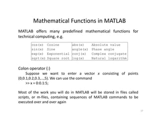
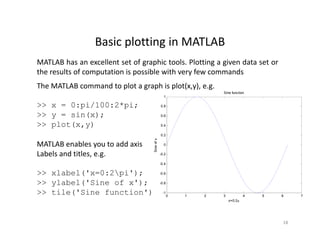
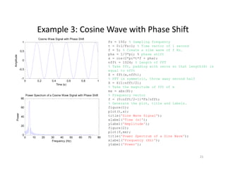
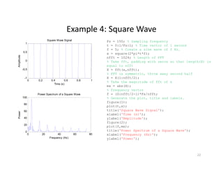
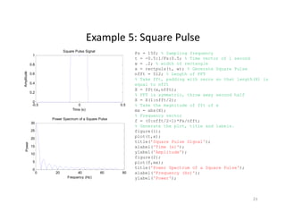
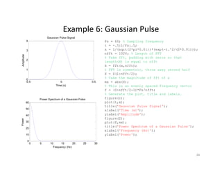
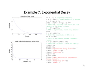
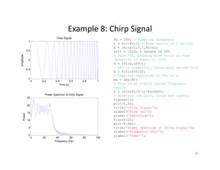
The document provides a comprehensive overview of the Fast Fourier Transform (FFT) and its implementation in MATLAB, explaining key concepts in signal processing, including continuous and discrete signals, periodicity, and frequency analysis. It outlines the necessity of transforming signals between time and frequency domains using the Fourier Transform and details how the FFT algorithm improves computation efficiency. Additionally, it introduces MATLAB functionalities, focusing on its mathematical operations and plotting capabilities to assist in implementing these concepts.

1. Fast Fourier Transform and
MATLAB Implementation
by
Wanjun Huang
forfor
Dr. Duncan L. MacFarlane
1

2. Signals
In the fields of communications, signal processing, and in electrical engineering
more generally, a signal is any time‐varying or spatial‐varying quantity
This variable(quantity) changes in time
• Speech or audio signal: A sound amplitude that varies in time
• Temperature readings at different hours of a day
• Stock price changes over days
• Etc• Etc.
Signals can be classified by continues‐time signal and discrete‐time signal:
• A discrete signal or discrete‐time signal is a time series, perhaps a signal that
h b l d f ti ti i lhas been sampled from a continuous‐time signal
• A digital signal is a discrete‐time signal that takes on only a discrete set of
values 1
Continuous Time Signal
1
Discrete Time Signal
-0.5
0
0.5
f(t)
-0.5
0
0.5
f[n]
0 10 20 30 40
-1
Time (sec)
0 10 20 30 40
-1
n
2

3. Periodic Signal
periodic signal and non‐periodic signal:
1
Periodic Signal
1
Non-Periodic Signal
0 10 20 30 40
-1
0
f(t)
Time (sec)
0 10 20 30 40
-1
0
f[n]
nn
• Period T: The minimum interval on which
a signal repeats
• Fundamental frequency: f0=1/TFundamental frequency: f0 1/T
• Harmonic frequencies: kf0
• Any periodic signal can be approximated
by a sum of many sinusoids at harmonic frequencies of the signal(kf0) with y y q g ( f0)
appropriate amplitude and phase
• Instead of using sinusoid signals, mathematically, we can use the complex
exponential functions with both positive and negative harmonic frequencies
)cos()sin()exp( tjttj  Euler formula:
3

4. Time‐Frequency Analysis
• A signal has one or more frequencies in it, and can be viewed from
two different standpoints: Time domain and Frequency domain
Time Domian (Banded Wren Song)
0
1
Amplitude
Time Domian (Banded Wren Song)
1
2
Power
Frequency Domain
0 2 4 6 8
x 10
4
-1
Sample Number
A
0 200 400 600 800 1000 1200
0
Frequency (Hz)
Time‐domain figure: how a signal changes over time
Why frequency domain analysis?
g g g
Frequency‐domain figure: how much of the signal lies within each given
frequency band over a range of frequencies
Why frequency domain analysis?
• To decompose a complex signal into simpler parts to facilitate analysis
• Differential and difference equations and convolution operations in the
time domain become algebraic operations in the frequency domain
• Fast Algorithm (FFT)
4

5. Fourier TransformFourier Transform
We can go between the time domain and the frequency domain
by using a tool called Fourier transform
• A Fourier transform converts a signal in the time domain to the
frequency domain(spectrum)
A i F i f h f d i
y g f
• An inverse Fourier transform converts the frequency domain
components back into the original time domain signal
Continuous‐Time Fourier Transform:



dejFtf tj



)(
2
1
)(



dtetfjF tj
 )()(
Continuous Time Fourier Transform:
Discrete‐Time Fourier Transform(DTFT):Discrete Time Fourier Transform(DTFT):




 2
)(
2
1
][ deeXnx njj




n
njj
enxeX 
][)(
5

6. Fourier Representation For Four Types of SignalsFourier Representation For Four Types of Signals
The signal with different time‐domain characteristics has different
frequency‐domain characteristics
1 Continues‐time periodic signal ‐‐‐> discrete non‐periodic
spectrum
q y
p
2 Continues‐time non‐periodic signal ‐‐‐> continues non‐periodic
spectrum
3 Discrete non‐periodic signal ‐‐‐> continues periodic spectrum3 Discrete non periodic signal > continues periodic spectrum
4 Discrete periodic signal ‐‐‐> discrete periodic spectrum
The last transformation between time‐domain and frequency is most q y
useful
The reason that discrete is associated with both time‐domain and frequency
domain is because computers can only take finite discrete time signalsp y g
6

7. Periodic SequencePeriodic Sequence
)(~)(~ kNnxnx  , where k is integer
A periodic sequence with period N is defined as:
Periodic
, g
kn
N
j
kn
N eW
2

For example:
)()( NnknNkkn
WWW 
(it is called Twiddle Factor)
Properties: Periodic )()( Nnk
N
nNk
N
kn
N WWW 

Symmetric )()(*
)( nNk
N
nkN
N
kn
N
kn
N WWWW 

Properties:
Orthogonal 

 


 other
rNnN
W
N
k
kn
N
0
1
0
For a periodic sequence with period N, only N samples
are independent. So that N sample in one period is enough to
represent the whole sequence
x(n)
represent the whole sequence
7

8. Discrete Fourier Series(DFS)Discrete Fourier Series(DFS)
Periodic signals may be expanded into a series of sine and
cosine functions






1
0
1
0
)(
~1
)(~
)(~)(
~
N
kn
N
N
n
kn
N
WkX
N
nx
WnxkX
cosine functions
))(
~
()(~
))(~()(
~
kXIDFSnx
nxDFSkX


 0nN
is still a periodic sequence with period N in frequency
domain
)(
~
kX
The Fourier series for the discrete‐time periodic wave shown below:
1
Sequence x (in time domain)
0.2
Fourier Coeffients
0
0.5
Amplitude
0 4
-0.2
0
X
0 10 20 30 40
0
time
0 10 20 30 40
-0.4
8

9. Finite Length SequenceFinite Length Sequence
 )(nx Nn 10 
Real lift signal is generally a
fi i l h
If we periodic extend it by the period N then  

rNnxnx )()(~




0
)(
)(
nx
nx
others
Nn 10 
finite length sequence
If we periodic extend it by the period N, then  
r
rNnxnx )()(
)(nx
)(~ nx
 
9

10. Relationship Between Finite Length Sequence
d P i di Sand Periodic Sequence
A periodic sequence is the periodic extension of a finite length
A finite length sequence is the principal value interval of the periodic
sequence
 

m
NnxrNnxnx ))(()()(~
A finite length sequence is the principal value interval of the periodic
sequence
)()(~)( nRnxnx N




0
1
)(nRN
others
Nn 10 
Where
0 others
So that:
)()](
~
[)()(~)( nRkXIDFSnRnxnx NN 
)()](~[)()(
~
)(
)()]([)()()(
nRnxDFSkRkXkX NN
NN

10

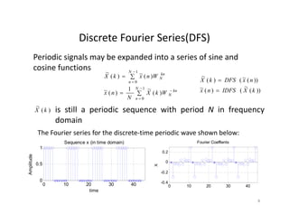
11. Discrete Fourier Transform(DFT)Discrete Fourier Transform(DFT)
• Using the Fourier series representation we have Discrete
Fourier Transform(DFT) for finite length signalFourier Transform(DFT) for finite length signal
• DFT can convert time‐domain discrete signal into frequency‐
domain discrete spectrum
Assume that we have a signal . Then the DFT of the
signal is a sequence for
1
0]}[{ 

N
nnx
][kX 1,,0  Nk 




1
0
/2
][][
N
n
Njnk
enxkX 
The Inverse Discrete Fourier Transform(IDFT):
 


1
0
/2
.1,,2,0,][
1
][
N
k
Njnk
NnekX
N
nx 
Note that because MATLAB cannot use a zero or negativeNote that because MATLAB cannot use a zero or negative
indices, the index starts from 1 in MATLAB
11

12. DFT ExampleDFT Example
The DFT is widely used in the fields of spectral analysis,
acoustics medical imaging and telecommunicationsacoustics, medical imaging, and telecommunications.
4
5
6
e
Time domain signal
For example:
0
1
2
3
Amplitude
)3,2,1,0(,4],6142[][  nNnx
nk
nkj
jnxenxkX )(][][][
3
0
2
3
0



0 0.5 1 1.5 2 2.5 3
-1
Time
nn 00 
116)1(42]0[ X
jjjX 2361)4(2]1[  10
12
Frequency domain signal
96)1()4(2]2[ X
jjjX 2361)4(2]3[ 
4
6
8
10
|X[k]|
0 0.5 1 1.5 2 2.5 3
0
2
Frequency 12

13. Fast Fourier Transform(FFT)Fast Fourier Transform(FFT)
• The Fast Fourier Transform does not refer to a new or different
type of Fourier transform. It refers to a very efficient algorithm foryp y g
computing the DFT
• The time taken to evaluate a DFT on a computer depends
principally on the number of multiplications involved. DFT needsprincipally on the number of multiplications involved. DFT needs
N2 multiplications. FFT only needs Nlog2(N)
• The central insight which leads to this algorithm is the
realization that a discrete Fourier transform of a sequence of Nrealization that a discrete Fourier transform of a sequence of N
points can be written in terms of two discrete Fourier transforms
of length N/2
• Thus if N is a power of two it is possible to recursively applyThus if N is a power of two, it is possible to recursively apply
this decomposition until we are left with discrete Fourier
transforms of single points
13

14. Fast Fourier Transform(cont.)Fast Fourier Transform(cont.)
Re‐writing 



1
0
/2
][][
N
n
Njnk
enxkX 
as 


1
0
][][
N
n
nk
NWnxkX
It is easy to realize that the same values of are calculated many times as thenk
WIt is easy to realize that the same values of are calculated many times as the
computation proceeds
Using the symmetric property of the twiddle factor, we can save lots of computations
NW
111 NNN
)12()2(
)()(][][
12
)12(
12
2
1
0
1
0
1
0
WrxWrx
WnxWnxWnxkX
N
rk
N
N
kr
N
N
nodd
n
kn
N
N
neven
n
kn
N
N
n
nk
N
  
 









)()(
)()(
)12()2(
12
0
22
12
0
21
00
kXWkX
WrxWWrx
WrxWrx
k
N
r
kr
N
k
N
N
r
kr
N
r
N
r
N
 
  





)()( 21 kXWkX k
N
Thus the N‐point DFT can be obtained from two N/2‐point transforms, one on even
input data, and one on odd input data.
14

15. Introduction for MATLABIntroduction for MATLAB
MATLAB is a numerical computing environment developed by
MathWorks. MATLAB allows matrix manipulations, plotting ofp , p g
functions and data, and implementation of algorithms
Getting helpGetting help
You can get help by typing the commands help or lookfor at
the >> prompt, e.g.
>> help fft>> help fft
Arithmetic operators
Symbol Operation Example
+ Addition 3 1 + 9+ Addition 3.1 + 9
‐ Subtraction 6.2 – 5
* Multiplication 2 * 3
/ Division 5 / 2/ Division 5 / 2
^ Power 3^2
15

16. Data Representations in MATLABData Representations in MATLAB
Variables: Variables are defined as the assignment operator “=” . The syntax of
variable assignment is
i bl l ( i )variable name = a value (or an expression)
For example,
>> x = 5
x =
5
>> y = [3*7, pi/3]; % pi is in MATLAB
Vectors/Matrices MATLAB can create and manip late arra s of 1 ( ectors) 2

Vectors/Matrices: MATLAB can create and manipulate arrays of 1 (vectors), 2
(matrices), or more dimensions
row vectors: a = [1, 2, 3, 4] is a 1X4 matrix
column vectors: b = [5; 6; 7; 8; 9] is a 5X1 matrix, e.g.
>> A = [1 2 3; 7 8 9; 4 5 6]
A = 1 2 3
7 8 9
4 5 64 5 6
16

17. Mathematical Functions in MATLABMathematical Functions in MATLAB
MATLAB offers many predefined mathematical functions for
technical computing, e.g.p g, g
cos(x) Cosine abs(x) Absolute value
sin(x) Sine angle(x) Phase angle
exp(x) Exponential conj(x) Complex conjugate
Colon operator (:)
exp(x) Exponential conj(x) Complex conjugate
sqrt(x) Square root log(x) Natural logarithm
Colon operator (:)
Suppose we want to enter a vector x consisting of points
(0,0.1,0.2,0.3,…,5). We can use the command
>> x = 0:0.1:5;;
Most of the work you will do in MATLAB will be stored in files called
scripts, or m‐files, containing sequences of MATLAB commands to be
executed over and over again
17

18. Basic plotting in MATLABBasic plotting in MATLAB
MATLAB has an excellent set of graphic tools. Plotting a given data set or
the results of computation is possible with very few commands
The MATLAB command to plot a graph is plot(x,y), e.g.
>> x = 0:pi/100:2*pi; 0.8
1
Sine function
p / p ;
>> y = sin(x);
>> plot(x,y)
0.2
0.4
0.6
x
MATLAB enables you to add axis
Labels and titles, e.g.
i
-0.4
-0.2
0
Sineofx
>> xlabel('x=0:2pi');
>> ylabel('Sine of x');
>> tile('Sine function') 0 1 2 3 4 5 6 7
-1
-0.8
-0.6
x=0:2x 0:2
18

19. Example 1: Sine WaveExample 1: Sine Wave
0.5
1
Sine Wave Signal
Fs = 150; % Sampling frequency
t = 0:1/Fs:1; % Time vector of 1 second
f = 5; % Create a sine wave of f Hz.
i (2* i*t*f)
-0.5
0
Amplitude
x = sin(2*pi*t*f);
nfft = 1024; % Length of FFT
% Take fft, padding with zeros so that length(X)
is equal to nfft
X = fft(x,nfft);
% FFT is symmetric, throw away second half
0 0.2 0.4 0.6 0.8 1
-1
Time (s)
80
Power Spectrum of a Sine Wave
% FFT is symmetric, throw away second half
X = X(1:nfft/2);
% Take the magnitude of fft of x
mx = abs(X);
% Frequency vector
f = (0:nfft/2-1)*Fs/nfft;
40
60
80
Power
% Generate the plot, title and labels.
figure(1);
plot(t,x);
title('Sine Wave Signal');
xlabel('Time (s)');
l b l('A lit d ')
0 10 20 30 40 50 60 70 80
0
20
Frequency (Hz)
P
ylabel('Amplitude');
figure(2);
plot(f,mx);
title('Power Spectrum of a Sine Wave');
xlabel('Frequency (Hz)');
ylabel('Power');Frequency (Hz) ylabel( Power );
19

20. Example 2: Cosine WaveExample 2: Cosine Wave
Fs = 150; % Sampling frequency
t = 0:1/Fs:1; % Time vector of 1 second
f = 5; % Create a sine wave of f Hz.
x = cos(2*pi*t*f);
0.5
1
Cosine Wave Signal
x = cos(2*pi*t*f);
nfft = 1024; % Length of FFT
% Take fft, padding with zeros so that length(X) is
equal to nfft
X = fft(x,nfft);
% FFT is symmetric, throw away second half
-0.5
0
Amplitude
y , y
X = X(1:nfft/2);
% Take the magnitude of fft of x
mx = abs(X);
% Frequency vector
f = (0:nfft/2-1)*Fs/nfft;
0 0.2 0.4 0.6 0.8 1
-1
Time (s)
80
Power Spectrum of a Cosine Wave
% Generate the plot, title and labels.
figure(1);
plot(t,x);
title('Sine Wave Signal');
xlabel('Time (s)');
ylabel('Amplitude');
40
60
80
Power
ylabel( Amplitude );
figure(2);
plot(f,mx);
title('Power Spectrum of a Sine Wave');
xlabel('Frequency (Hz)');
ylabel('Power');
0 10 20 30 40 50 60 70 80
0
20
Frequency (Hz)
P
yFrequency (Hz)
20

21. Example 3: Cosine Wave with Phase ShiftExample 3: Cosine Wave with Phase Shift
Fs = 150; % Sampling frequency
t = 0:1/Fs:1; % Time vector of 1 second
f = 5; % Create a sine wave of f Hz.
pha = 1/3*pi; % phase shift
0.5
1
Cosine Wave Signal with Phase Shift
pha = 1/3*pi; % phase shift
x = cos(2*pi*t*f + pha);
nfft = 1024; % Length of FFT
% Take fft, padding with zeros so that length(X) is
equal to nfft
X = fft(x,nfft);
-0.5
0
Amplitude
( , )
% FFT is symmetric, throw away second half
X = X(1:nfft/2);
% Take the magnitude of fft of x
mx = abs(X);
% Frequency vector
/ /
0 0.2 0.4 0.6 0.8 1
-1
Time (s)
80
Power Spectrum of a Cosine Wave Signal with Phase Shift
f = (0:nfft/2-1)*Fs/nfft;
% Generate the plot, title and labels.
figure(1);
plot(t,x);
title('Sine Wave Signal');
xlabel('Time (s)');
40
60
80
Power
xlabel( Time (s) );
ylabel('Amplitude');
figure(2);
plot(f,mx);
title('Power Spectrum of a Sine Wave');
xlabel('Frequency (Hz)');
0 10 20 30 40 50 60 70 80
0
20
Frequency (Hz)
P
q y
ylabel('Power');
Frequency (Hz)
21

22. Example 4: Square WaveExample 4: Square Wave
0.5
1
Square Wave Signal Fs = 150; % Sampling frequency
t = 0:1/Fs:1; % Time vector of 1 second
f = 5; % Create a sine wave of f Hz.
x = square(2*pi*t*f);
-0.5
0
Amplitude
x = square(2*pi*t*f);
nfft = 1024; % Length of FFT
% Take fft, padding with zeros so that length(X) is
equal to nfft
X = fft(x,nfft);
% FFT is symmetric, throw away second half
0 0.2 0.4 0.6 0.8 1
-1
Time (s)
100
Power Spectrum of a Square Wave
y , y
X = X(1:nfft/2);
% Take the magnitude of fft of x
mx = abs(X);
% Frequency vector
f = (0:nfft/2-1)*Fs/nfft;
40
60
80
100
Power
% Generate the plot, title and labels.
figure(1);
plot(t,x);
title('Square Wave Signal');
xlabel('Time (s)');
ylabel('Amplitude');
0 20 40 60 80
0
20
40
Frequency (Hz)
ylabel( Amplitude );
figure(2);
plot(f,mx);
title('Power Spectrum of a Square Wave');
xlabel('Frequency (Hz)');
ylabel('Power');y
22

23. Example 5: Square PulseExample 5: Square Pulse
0.8
1
Square Pulse Signal
Fs = 150; % Sampling frequency
t = -0.5:1/Fs:0.5; % Time vector of 1 second
w = .2; % width of rectangle
x = rectpuls(t w); % Generate Square Pulse
0.2
0.4
0.6
Amplitude
x = rectpuls(t, w); % Generate Square Pulse
nfft = 512; % Length of FFT
% Take fft, padding with zeros so that length(X) is
equal to nfft
X = fft(x,nfft);
% FFT is symmetric, throw away second half
-0.5 0 0.5
0
Time (s)
30
Power Spectrum of a Square Pulse
y , y
X = X(1:nfft/2);
% Take the magnitude of fft of x
mx = abs(X);
% Frequency vector
f = (0:nfft/2-1)*Fs/nfft;
15
20
25
Power
% Generate the plot, title and labels.
figure(1);
plot(t,x);
title('Square Pulse Signal');
xlabel('Time (s)');
ylabel('Amplitude');
0 20 40 60 80
0
5
10
Frequency (Hz)
ylabel( Amplitude );
figure(2);
plot(f,mx);
title('Power Spectrum of a Square Pulse');
xlabel('Frequency (Hz)');
ylabel('Power');y
23

24. Example 6: Gaussian PulseExample 6: Gaussian Pulse
3
4
Gaussian Pulse Signal
Fs = 60; % Sampling frequency
t = -.5:1/Fs:.5;
x = 1/(sqrt(2*pi*0.01))*(exp(-t.^2/(2*0.01)));
nfft = 1024; % Length of FFT
1
2
Amplitude
nfft = 1024; % Length of FFT
% Take fft, padding with zeros so that
length(X) is equal to nfft
X = fft(x,nfft);
% FFT is symmetric, throw away second half
X = X(1:nfft/2);
-0.5 0 0.5
0
Time (s)
( )
% Take the magnitude of fft of x
mx = abs(X);
% This is an evenly spaced frequency vector
f = (0:nfft/2-1)*Fs/nfft;
% Generate the plot, title and labels.
40
50
60
Power Spectrum of a Gaussian Pulse
r
figure(1);
plot(t,x);
title('Gaussian Pulse Signal');
xlabel('Time (s)');
ylabel('Amplitude');
figure(2);
0
10
20
30
Power
figure(2);
plot(f,mx);
title('Power Spectrum of a Gaussian Pulse');
xlabel('Frequency (Hz)');
ylabel('Power');
0 5 10 15 20 25 30
0
Frequency (Hz)
24

25. Example 7: Exponential DecayExample 7: Exponential Decay
1.5
2
Exponential Decay Signal
Fs = 150; % Sampling frequency
t = 0:1/Fs:1; % Time vector of 1 second
x = 2*exp(-5*t);
nfft 1024 % Length of FFT
0.5
1
Amplitude
nfft = 1024; % Length of FFT
% Take fft, padding with zeros so that
length(X) is equal to nfft
X = fft(x,nfft);
% FFT is symmetric, throw away second
half
0 0.2 0.4 0.6 0.8 1
0
Time (s)
P S t f E ti l D Si l
half
X = X(1:nfft/2);
% Take the magnitude of fft of x
mx = abs(X);
% This is an evenly spaced frequency
vector
40
50
60
70
Power Spectrum of Exponential Decay Signal
er
f = (0:nfft/2-1)*Fs/nfft;
% Generate the plot, title and labels.
figure(1);
plot(t,x);
title('Exponential Decay Signal');
xlabel('Time (s)');
0 20 40 60 80
0
10
20
30
Powe
xlabel('Time (s)');
ylabel('Amplitude');
figure(2);
plot(f,mx);
title('Power Spectrum of Exponential
Decay Signal');
0 20 40 60 80
Frequency (Hz)
y g );
xlabel('Frequency (Hz)');
ylabel('Power');
25

26. Example 8: Chirp SignalExample 8: Chirp Signal
0.5
1
Chirp Signal
Fs = 200; % Sampling frequency
t = 0:1/Fs:1; % Time vector of 1 second
x = chirp(t,0,1,Fs/6);
nfft = 1024; % Length of FFT
-0.5
0
Amplitude
; g
% Take fft, padding with zeros so that
length(X) is equal to nfft
X = fft(x,nfft);
% FFT is symmetric, throw away second half
X = X(1:nfft/2);
0 0.2 0.4 0.6 0.8 1
-1
Time (s)
Power Spectrum of Chirp Signal
% Take the magnitude of fft of x
mx = abs(X);
% This is an evenly spaced frequency
vector
f = (0:nfft/2-1)*Fs/nfft;
% Generate the plot title and labels
15
20
25
p p g
wer
% Generate the plot, title and labels.
figure(1);
plot(t,x);
title('Chirp Signal');
xlabel('Time (s)');
ylabel('Amplitude');
0 20 40 60 80 100
0
5
10
Pow
y p
figure(2);
plot(f,mx);
title('Power Spectrum of Chirp Signal');
xlabel('Frequency (Hz)');
ylabel('Power');
Frequency (Hz)
26