Design of FFT Processor

.. Report by Rohit Singh and Amit Kumar Singh for Self –Study-Course, M.Tech. (VST),
Deptt. Of EE,SOE, Shiv Nadar University
1
IMPLEMENTATION OF FAST FOURIER
TRANSFORM
Self Study Course
By
Rohit Singh
Amit Kumar Singh
(M.Tech (VST))

2
Contents
1. Introduction to fast fourier transform ...………………… 03
2. Butterfly structures for FFT ...………………… 08
3. Implementation of 16-point FFT blocks …………………... 11
4. Matlab code for DFT …………………. 12
5. Matlab code for 8 point FFT …………………. 13
6. VHDL code for 16 point FFT Processor …………… 14

3
1. INTRODUCTION TO FAST FOURIER TRANSFORM
A Fast Fourier Transform (FFT) is an efficient algorithm to compute the Discrete
Fourier Transform (DFT) and its inverse. There are many distinct FFT algorithms
involving a wide range of mathematics, from simple complex-number arithmetic to group
theory and number theory. The fast Fourier Transform is a highly efficient procedure for
computing the DFT of a finite series and requires less number of computations than that
of direct evaluation of DFT. It reduces the computations by taking advantage of the fact
that the calculation of the coefficients of the DFT can be carried out iteratively. Due to
this, FFT computation technique is used in digital spectral analysis, filter simulation,
autocorrelation and pattern recognition.
The FFT is based on decomposition and breaking the transform into smaller
transforms and combining them to get the total transform. FFT reduces the computation
time required to compute a discrete Fourier transform and improves the performance by a
factor of 100 or more over direct evaluation of the DFT.
A DFT decomposes a sequence of values into components of different
frequencies. This operation is useful in many fields but computing it directly from the
definition is often too slow to be practical. An FFT is a way to compute the same result
more quickly: computing a DFT of N points in the obvious way, using the definition,
takes O( N2
) arithmetical operations, while an FFT can compute the same result in only
O(N log N) operations.
The difference in speed can be substantial, especially for long data sets where N
may be in the thousands or millions—in practice, the computation time can be reduced by
several orders of magnitude in such cases, and the improvement is roughly proportional
to N /log (N). This huge improvement made many DFT-based algorithms practical. FFT’s
are of great importance to a wide variety of applications, from digital signal processing

4
and solving partial differential equations to algorithms for quick multiplication of large
integers.
The most well known FFT algorithms depend upon the factorization of N, but
there are FFT with O (N log N) complexity for all N, even for prime N. Many FFT
algorithms only depend on the fact that is an N th primitive root of unity, and thus can be
applied to analogous transforms over any finite field, such as number-theoretic
transforms.
The Fast Fourier Transform algorithm exploit the two basic properties of the
twiddle factor - the symmetry property and periodicity property which reduces the
number of complex multiplications required to perform DFT.
FFT algorithms are based on the fundamental principle of decomposing the
computation of discrete Fourier Transform of a sequence of length N into successively
smaller discrete Fourier transforms. There are basically two classes of FFT algorithms.
A) Decimation In Time (DIT) algorithm
B) Decimation In Frequency (DIF) algorithm.
In decimation-in-time, the sequence for which we need the DFT is successively
divided into smaller sequences and the DFTs of these subsequences are combined in a
certain pattern to obtain the required DFT of the entire sequence. In the decimation-in-
frequency approach, the frequency samples of the DFT are decomposed into smaller and
smaller subsequences in a similar manner.
The number of complex multiplication and addition operations required by the
simple forms both the Discrete Fourier Transform (DFT) and Inverse Discrete Fourier
Transform (IDFT) is of order N2
as there are N data points to calculate, each of which
requires N complex arithmetic operations.
The discrete Fourier transform (DFT) is defined by the formula:

5
;
2
1
0
)()( N
nKj
N
n
enxKX





Where K is an integer ranging from 0 to N − 1.
The algorithmic complexity of DFT will O(N2
) and hence is not a very efficient
method. If we can't do any better than this then the DFT will not be very useful for the
majority of practical DSP application. However, there are a number of different 'Fast
Fourier Transform' (FFT) algorithms that enable the calculation the Fourier transform of
a signal much faster than a DFT. As the name suggests, FFTs are algorithms for quick
calculation of discrete Fourier transform of a data vector. The FFT is a DFT algorithm
which reduces the number of computations needed for N points from O(N2
) to O(N log N)
where log is the base-2 logarithm. If the function to be transformed is not harmonically
related to the sampling frequency, the response of an FFT looks like a ‘sinc’ function (sin
x) / x.
The Radix-2 DIT algorithm rearranges the DFT of the function xn into two parts:
a sum over the even-numbered indices n = 2m and a sum over the odd-numbered indices
n = 2m + 1:

6
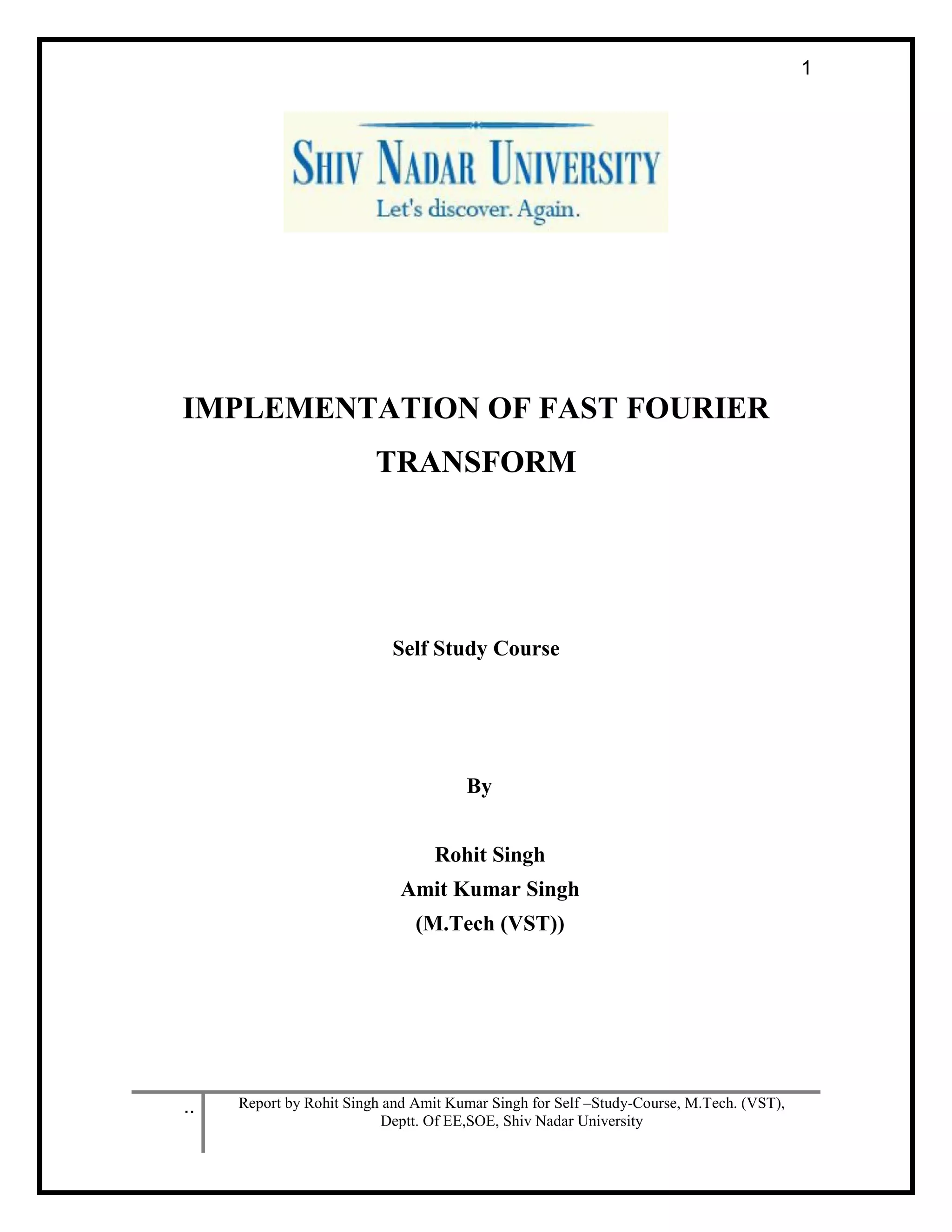
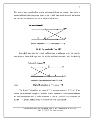
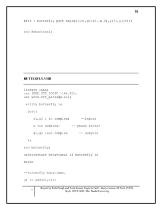
One can factor a common multiplier out of the second sum in the
equation. It is the two sums are the DFT of the even-indexed part x2m and the DFT of
odd-indexed part x2m + 1 of the function xn. Denote the DFT of the Even-indexed inputs
x2m by Ek and the DFT of the Odd-indexed inputs x2m + 1 by Ok and we obtain:
However, these smaller DFTs have a length of N/2, so we need compute only N/2
outputs: thanks to the periodicity properties of the DFT, the outputs for N/2 < k < N from
a DFT of length N/2 are identical to the outputs for 0< k < N/2. That is, Ek + N / 2 = Ek
and Ok + N / 2 = Ok. The phase factor exp[ − 2πik / N] called a twiddle factor which
obeys the relation: exp[ − 2πi(k + N / 2) / N] = e − πiexp[ − 2πik / N] = − exp[ − 2πik / N],
flipping the sign of the Ok + N / 2 terms. Thus, the whole DFT can be calculated as
follows:
This result, expressing the DFT of length N recursively in terms of two DFTs of
size N/2, is the core of the radix-2 DIT fast Fourier transform. The algorithm gains its
speed by re-using the results of intermediate computations to compute multiple DFT
outputs. Note that final outputs are obtained by a +/− combination of Ek and Okexp( −
2πik / N), which is simply a size-2 DFT; when this is generalized to larger radices below,
the size-2 DFT is replaced by a larger DFT (which itself can be evaluated with an FFT).

7
This process is an example of the general technique of divide and conquers algorithms. In
many traditional implementations, however, the explicit recursion is avoided, and instead
one traverses the computational tree in breadth-first fashion.
Fig 1.1 Decimation In Time FFT
In the DIT algorithm, the twiddle multiplication is performed before the butterfly
stage whereas for the DIF algorithm, the twiddle multiplication comes after the Butterfly
stage. Fig 1.2 Decimation In Frequency FFT
The 'Radix 2' algorithms are useful if N is a regular power of 2 (N=2p). If we
assume that algorithmic complexity provides a direct measure of execution time and that
the relevant logarithm base is 2 then as shown in table 1.1, ratio of execution times for
the (DFT) vs. (Radix 2 FFT) increases tremendously with increase in N.

8
The term 'FFT' is actually slightly ambiguous, because there are several
commonly used 'FFT' algorithms. There are two different Radix 2 algorithms, the so-
called 'Decimation in Time' (DIT) and 'Decimation in Frequency' (DIF) algorithms. Both
of these rely on the recursive decomposition of an N point transform into 2 (N/2) point
transforms.
Number
of Points,
N
Complex Multiplications
in Direct computations,
N2
Complex Multiplication
in FFT Algorithm, (N/2)
log2 N
Speed
improvement
Factor
4 16 4 4.0
8 64 12 5.3
16 256 32 8.0
32 1024 80 12.8
64 4096 192 21.3
128 16384 448 36.6
Table 1.1: Comparison of Execution Times, DFT & Radix – 2 FFT
2. BUTTERFLY STRUCTURES FOR FFT
Basically FFT algorithms are developed by means of divide and conquer method,
the is depending on the decomposition of an N point DFT in to smaller DFT’s. If N is
factored as N = r1,r2,r3 ..rL where r1=r2=…=rL=r, then rL =N. where r is called as Radix of
FFT algorithm.
If r= 2, then it is called as radix-2 FFT algorithm,. The basic DFT is of size of 2.
The N point DFT is decimated into 2 point DFT by two ways such as Decimation In
Time (DIT) and Decimation In Frequency (DIF) algorithm. Both the algorithm take the
advantage of periodicity and symmetry property of the twiddle factor.
N
nKj
enK
N
W


2

9
The radix-2 decimation-in-frequency FFT is an important algorithm obtained by
the divide and conquers approach. The Fig. 1.3 below shows the first stage of the 8-point
DIF algorithm.
Fig. 1.3 First Stage of 8 point Decimation in Frequency Algorithm.
The decimation, however, causes shuffling in data. The entire process involves v
= log2 N stages of decimation, where each stage involves N/2 butterflies of the type
shown in the Fig. 1.3.
Fig. 1.4: Butterfly Scheme.

10
Here N
nkj
ek
nW


2
is the Twiddle factor.
Consequently, the computation of N-point DFT via this algorithm requires (N/2)
log2 N complex multiplications. For illustrative purposes, the eight-point decimation-in
frequency algorithm is shown in the Figure below. We observe, as previously stated, that
the output sequence occurs in bit-reversed order with respect to the input. Furthermore, if
we abandon the requirement that the computations occur in place, it is also possible to
have both the input and output in normal order. The 8 point Decimation In frequency
algorithm is shown in Fig 1.5.
Fig. 1.5 8 point Decimation in Frequency Algorithm

11
3. IMPLEMENTATION OF 16-POINT FFT BLOCKS
The FFT computation is accomplished in three stages. The x(0) until x(15)
variables are denoted as the input values for FFT computation and X(0) until X(15) are
denoted as the outputs. The pipeline architecture of the 16 point FFT is shown in Fig 2.1
consisting of butterfly schemes in it. There are two operations to complete the
computation in each stage.
Fig 2.1: Architecture of 16 point FFT.
The upward arrow will execute addition operation while downward arrow will
execute subtraction operation. The subtracted value is multiplied with twiddle factor

12
value before being processed into the next stage. This operation is done concurrently and
is known as butterfly process.
4. Matlab Code for DFT
% program to calculate DFT.
clear all;
clc;
x=input ('enter the sequence ');
tic
N=size(x,2);
w=zeros(N);
for a=1:N
for b=1:N
w(a,b)=exp((-1j*2*pi*(a-1)*(b-1))/N);
end
end
Xk = w*x';
Xk
Toc

13
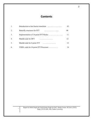
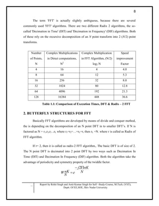
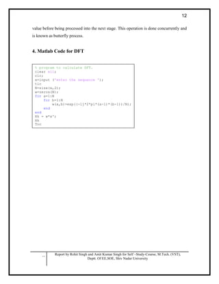
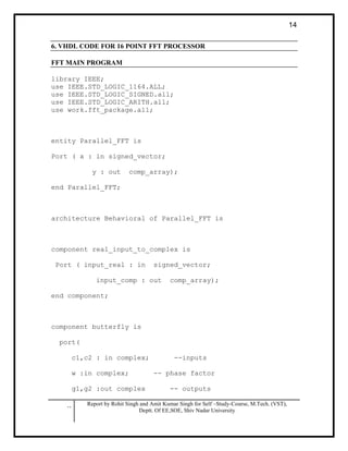
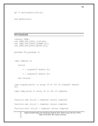
5. Matlab Code for 8 point FFT
% program to calculate 8 point FFT
clear all;
clc;
x=input (' enter the sequence of length 8 ');
tic
s0=zeros(1,8);
s1=zeros(1,8);
s2=zeros(1,8);
s3=zeros(1,8);
N=size(x,2);
if (N < 8 || N > 8)
disp(' sequence is of not proper length ');
else
stage1=[1 1 1 0-1j 1 1 1 0-1j];
stage2=[1 1 1 1 1 0.707-0.707j 0-1j -0.707-0.707j];
p=[0:7]';
t=bitrevorder(p);
% calculation of stage zero
for i=1:N
s0(i)=x(t(i)+1);
end
% calculation of stage one
for i=1:2:N
s1(i)=s0(i)+s0(i+1);
s1(i+1)=s0(i)-s0(i+1);
end
for a=1:N
s1(a)=s1(a)*stage1(a);
end
% calculation of stage two
for i=1:4:N
s2(i)=s1(i)+s1(i+2);
s2(i+1)=s1(i+1)+s1(i+3);
s2(i+2)=s1(i)-s1(i+2);
s2(i+3)=s1(i+1)-s1(i+3);
end
for a=1:N
s2(a)=s2(a)*stage2(a);
end
% calculation of stage three
s3(1)=s2(1)+s2(5);
s3(2)=s2(2)+s2(6);
s3(3)=s2(3)+s2(7);
s3(4)=s2(4)+s2(8);
s3(5)=s2(1)-s2(5);
s3(6)=s2(2)-s2(6);
s3(7)=s2(3)-s2(7);
s3(8)=s2(4)-s2(8);
end
disp(' FFT result ');
s3
toc

14
6. VHDL CODE FOR 16 POINT FFT PROCESSOR
FFT MAIN PROGRAM
library IEEE;
use IEEE.STD_LOGIC_1164.ALL;
use IEEE.STD_LOGIC_SIGNED.all;
use IEEE.STD_LOGIC_ARITH.all;
use work.fft_package.all;
entity Parallel_FFT is
Port ( x : in signed_vector;
y : out comp_array);
end Parallel_FFT;
architecture Behavioral of Parallel_FFT is
component real_input_to_complex is
Port ( input_real : in signed_vector;
input_comp : out comp_array);
end component;
component butterfly is
port(
c1,c2 : in complex; --inputs
w :in complex; -- phase factor
g1,g2 :out complex -- outputs

15
);
end component;
constant w : comp_array := (
("0100000000000000", "0000000000000000"),
("0011101100100001", "1110011110000010"),
("0010110101000001", "1101001010111111"),
("0001100001111110", "1100010011011111"),
("0000000000000000", "1100000000000000"),
("1110011110000010", "1100010011011111"),
("1101001010111111", "1101001010111111"),
("1100010011011111", "1110011110000010"),
("1100000000000000", "0000000000000000"),
("1100010011011111", "0001100001111110"),
("1101001010111111", "0010110101000001"),
("1110011110000010", "0011101100100001"),
("0000000000000000", "0100000000000000"),
("0001100001111110", "0011101100100001"),
("0010110101000001", "0010110101000001"),
("0011101100100001", "0001100001111110")
);
signal s, g1, g2, g3 : comp_array := (others =>
("0000000000000000","0000000000000000"));

16
begin
--Real Input value transformed in complex value
sixteen_bits_complex_transform : real_input_to_complex port
map(x, s);
--first stage of butterfly's.
bf11 : butterfly port map(s(0),s(8),w(0),g1(0),g1(8));
--second stage of butterfly's.
bf21 : butterfly port map(g1(0),g1(4),w(0),g2(0),g2(4));

17
bf27 : butterfly port
map(g1(10),g1(14),w(4),g2(10),g2(14));
map(g1(11),g1(15),w(6),g2(11),g2(15));
--third stage of butterfly's.
map(g2(12),g2(14),w(0),g3(12),g3(14));
map(g2(13),g2(15),w(4),g3(13),g3(15));
--fourth stage of butterfly's.
bf41 : butterfly port map(g3(0),g3(1),w(0),y(0),y(8));

18
end Behavioral;
BUTTERFLY.VHD
library IEEE;
entity butterfly is
port(
c1,c2 : in complex; --inputs
w :in complex; -- phase factor
g1,g2 :out complex -- outputs
);
end butterfly;
architecture Behavioral of butterfly is
begin
--butterfly equations.
g1 <= add(c1,c2);

19
g2 <= mult(sub(c1,c2),w);
end Behavioral;
FFT PACKAGE
library IEEE;
package fft_package is
type complex is
record
r : signed(15 downto 0);
i : signed(15 downto 0);
end record;
type signed_vector is array (0 to 15) of signed(7 downto
0);
type comp_array is array (0 to 15) of complex;
function add (n1,n2 : complex) return complex;
function sub (n1,n2 : complex) return complex;
function mult (n1,n2 : complex) return complex;

20
end fft_package;
package body fft_package is
--addition of complex numbers
function add (n1,n2 : complex) return complex is
variable sum : complex;
begin
sum.r:=n1.r + n2.r;
sum.i:=n1.i + n2.i;
return sum;
end add;
--subtraction of complex numbers.
function sub (n1,n2 : complex) return complex is
variable diff : complex;
begin
diff.r:=n1.r - n2.r;
diff.i:=n1.i - n2.i;
return diff;
end sub;
--multiplication of complex numbers.
function mult (n1,n2 : complex) return complex is

21
variable prod : complex;
variable prod_aux_r : signed(31 downto 0);
variable prod_aux_i : signed(31 downto 0);
begin
prod_aux_r := (n1.r * n2.r) - (n1.i * n2.i);
prod.r:= prod_aux_r(29 downto 14);
prod_aux_i := (n1.r * n2.i) + (n1.i * n2.r);
prod.i:= prod_aux_i(29 downto 14);
return prod;
end mult;
end fft_package;
REAL TO COMPLEX
library IEEE;
entity real_input_to_complex is

22
Port ( input_real : in signed_vector;
input_comp : out comp_array);
end real_input_to_complex;
architecture Behavioral of real_input_to_complex is
component sig_ext_8_to_16_bits is
Port ( sig_in : in signed(7 downto 0);
sig_out : out complex);
end component;
begin
input0 : sig_ext_8_to_16_bits port map (input_real(0),
input_comp(0));
input_comp(1));
input_comp(2));
input_comp(3));
input_comp(4));
input_comp(5));
input_comp(6));
input_comp(7));

23
input_comp(8));
input_comp(9));
input_comp(10));
input_comp(11));
input_comp(12));
input_comp(13));
input_comp(14));
input_comp(15));
end Behavioral;
EIGHT TO SIXTEEN
library IEEE;

24
entity sig_ext_8_to_16_bits is
Port ( sig_in : in signed(7 downto 0);
sig_out : out complex);
end sig_ext_8_to_16_bits;
architecture Behavioral of sig_ext_8_to_16_bits is
signal sig_out_real : signed(15 downto 0);
begin
sig_out_real <= X"00" & sig_in when sig_in(7)='0' else
X"ff" & sig_in ;
sig_out <= (sig_out_real, "0000000000000000");
end Behavioral;
TEST BENCH
library IEEE;
ENTITY fft_cooley_tukey_tb IS
END fft_cooley_tukey_tb;

25
ARCHITECTURE behavior OF fft_cooley_tukey_tb IS
-- Component Declaration for the Unit Under Test (UUT)
COMPONENT Parallel_FFT
Port ( x : in signed_vector;
y : out comp_array);
END COMPONENT;
--Inputs
signal x : signed_vector:= (others => "00000000");
--Outputs
signal y : comp_array;
BEGIN
-- Instantiate the Unit Under Test (UUT)
uut: Parallel_FFT PORT MAP (
x => x,
y => y
);
-- Stimulus process
stim_proc: process

26
begin
-- hold reset state for 100 ns.
wait for 100 ns;
-- x<=("00000001",
-- "00000001",
-- "00000001",
-- "00000001",
-- "00000001",
-- "00000001",
-- "00000001",
-- "00000001",
-- "00000001",
-- "00000001",
-- "00000001",
-- "00000001",
-- "00000001",
-- "00000001",
-- "00000001",
-- "00000001"
-- );
-- x<=("00000000",

27
-- "00000000",
-- "00000000",
-- "00000000",
-- "00000000",
-- "00000000",
-- "00000000",
-- "00000000",
-- "00000001",
-- "00000001",
-- "00000001",
-- "00000001",
-- "00000001",
-- "00000001",
-- "00000001",
-- "00000001"
-- );
x<=("00000101",
"00001010",
"00001111",
"00010100",
"00011001",
"00011110",

28
"00100011",
"00101000",
"00101101",
"00110010",
"00110111",
"00111100",
"01000001",
"01000110",
"01001011",
"01010000"
);
wait;
end process;
END;

Design of FFT Processor

More Related Content

What's hot

Viewers also liked

Similar to Design of FFT Processor

More from Rohit Singh

Recently uploaded

Design of FFT Processor