This document outlines key concepts in linear models and estimation that will be covered in the STA721 Linear Models course, including:
1) Linear regression models decompose observed data into fixed and random components.
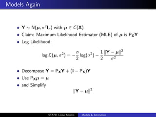
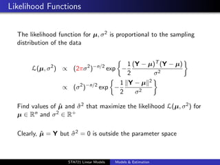
2) Maximum likelihood estimation finds parameter values that maximize the likelihood function.
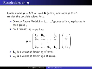
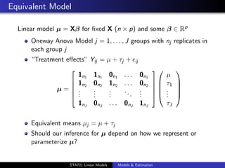
3) Linear restrictions on the mean vector μ define a subspace and equivalent parameterizations represent the same subspace.
4) Inference should be independent of the parameterization or coordinate system used to represent μ.

![Models
Take an random vector Y ∈ Rn which is observable and decompose
Y =µ+
into µ ∈ Rn (unknown, fixed) and ∈ Rn unobservable error
vector (random)
Usual assumptions?
E[ ] = 0 ⇒ E[Y] = µ (mean vector)
Cov[ ] = σ 2 In ⇒ Cov[Y] = σ 2 In (errors are uncorrelated)
∼ N(0, σ 2 I) ⇒ Y ∼ N(µ, σ 2 I)
The distribution assumption allows us to right down a likelihood
function
duke.eps
STA721 Linear Models Models & Estimation](https://image.slidesharecdn.com/models-120910144648-phpapp01/85/Models-3-320.jpg)
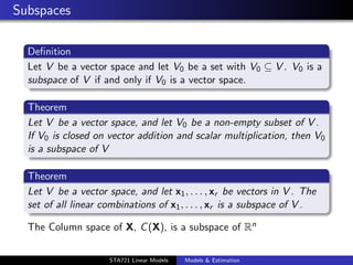
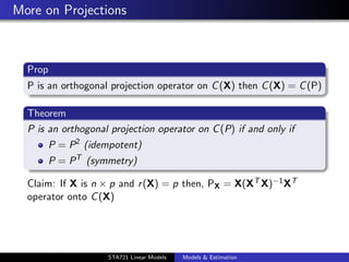
![Column Space
Many equivalent ways to represent the same mean vector –
inference should be independent of the coordinate system used
Let X1 , X2 , . . . , Xp ∈ Rn
The set of all linear combinations of X1 , . . . , Xp is the space
spanned by X1 , . . . , Xp ≡ S(X1 , . . . , Xp )
Let X = [X1 X2 . . . Xp ] be a n × p matrix with columns Xj
then the column space of X, C (X) = S(X1 , . . . , Xp ) space
spanned by the (column) vectors of X
µ ∈ C (X) : C (X) = {µ | µ ∈ Rn such that Xβ = µ for some
β ∈ Rp } (also called the Range of X, R(X)
β are the “coordinates” of µ in this space
C (X) is a subspace of Rn
duke.eps
STA721 Linear Models Models & Estimation](https://image.slidesharecdn.com/models-120910144648-phpapp01/85/Models-7-320.jpg)