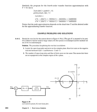
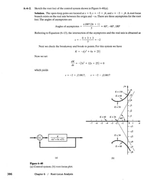
The document discusses root locus analysis and provides examples of solving for root loci of different control systems. It contains: 1) An example problem walking through the steps to sketch the root loci of a control system, including locating poles and zeros, finding breakaway/break-in points, and determining where loci cross the imaginary axis. 2) Additional example problems providing the solutions for sketching various other control system root loci, using the same procedure and noting how the system response depends on the location of closed-loop poles. 3) Details on how to determine asymptotes, departure angles, and intersection points used in the root locus analysis of different order systems.

1. Similarly, the program for the fourth-order transfer function approximation with
T = 0.1 sec is
[num,denl = pade(0.1, 4);
printsys(num,den, 'st)
numlden =
sA4 - 2O0sA3 + 180O0sA2 - 840000~+ 16800000
sA4 + 200sA3 + 18000sA2 + 840000s + 16800000
Notice that the pade approximation depends on the dead time T and the desired order
for the approximating transfer function.
EXAMPLE PROBLEMS AND SOLUTIONS
A-6-1. Sketch the root loci for the system shown in Figure 6-39(a). (The gain K is assumed to be posi-
tive.) Observe that for small or large values of K the system is overdamped and for medium val-
ues of K it is underdamped.
Solution. The procedure for plotting the root loci is as follows:
1. Locate the open-loop poles and zeros on the complex plane. Root loci exist on the negative
real axis between 0 and -1 and between -2 and -3.
2. The number of open-loop poles and that of finite zeros are the same.This means that there
are no asymptotes in the complex region of the s plane.
(2)
Figure 6-39
(a) Control system; (b) root-locus plot.
Chapter 6 / Root-Locus Analysis

2. 3. Determine the breakaway and break-in points.The characteristic equation for the system IS
The breakaway and break-in points are determined from
dK (2s + l ) ( s + 2 ) ( s + 3 ) - s(s + 1)(2>+ 5 )
- - --
rls [ ( s+ 2 ) ( s + 3)12
as follows:
Notice that both points are on root loci. Therefore, they are actual breakaway or break-in
points. At point s = -0.634, the value of K is
Similarly, at s = -2.36h,
(Because points = -0.634 lies between two poles,it is a breakaway point, and because point
s = -2.366 lies between two zeros, it is a break-in point.)
4. Determine a sufficient number of points t h d satisfy the angle condition. (It can he found
that the root loci involve a circle with center at -1.5 that passes through the breakaway and
break-in points.) The root-locus plot for this system is shown in Figure 6-3Y(h).
Note that this system is stable for m y positive value of K since all the root loci lie in the left-
half s plane.
Small kalues of I*: (0c K < 0.0718)correspond to an overdampcd system. Medium value
01' I< (0.0718 .-: K .;14) correspond to an underdamped system. Finally. large values ol
K ( 14 = K ) correspond to an overdamped systern.With a large value of K, the steady state can
be I-eachcdin much shorter time than with a mall value o f I<.
The value of K should be adjusted so thal system performance is optimum according to ;I
given performance index.
Example Problems and Solutions 385

3. A-6-2. Sketch the root loci of the control system shown in Figure 6-40(a).
Solution. The open-loop poles are located at s = 0, s = -3 + j4, and s = -3 - j4. A root locus
branch existson the real axis between the origin and -oo.There are three asymptotes for the root
1oci.The angles of asymptotes are
&18O0(2k+ 1)
Angles of asymptotes =
3
= 60°,-60°, 180"
Referring to Equation (6-13), the intersection of the asymptotes and the real axis is obtained as
Next we check the breakaway and break-in points. For this system we have
K = -s(s2 + 6s + 25)
Now we set
which yields
Figure 6-40
(a) Control system; (b) root-locus plot.
Chapter 6 / Root-LocusAnalysis

4. Notice that at points s = -2 * ~2.0817the ang!e condition is not satisfied. Hence, they are nei-
ther breakaway nor break-in points. In fact, if we calculate the value of K, we obtain
(To be an actual breakaway or break-in point, the corresponding value of K must be real and
positive.)
The angle of departure from the complex pole in the upper half s plane is
The points where root-locus branches cross the imaginary axis may be found by substituting
s = j w into the characteristic equation and solving the equation for w and K as follows: Noting
that the characteristic equation is
we have
which yields
Root-locus branches cross the imaginary axis at w = 5 and w = -S.The value of gain K at the
crossing points is 150.Also, the root-locus branch on the real axis touches the imaginary axis at
w = 0.Figure 6-40(b) shows a root-locus plot for the svstern.
It is noted that if the order of the numerator of G ( s ) H ( s )is lower than that of the denomi-
nator by two or more, and if some of the closed-looppoles move on the root locus toward the right
as gain K is increased, then other closed-loop poles must move toward the left as gain K is in-
creased.This fact can be seen clearly in this problem. If the gain K is increased from K = 34 to
K = 68,the complex-conjugate closed-loop poles are moved from s = -2 + 13.65 to s = -1 + j4:
the third pole is moved from s = -2 (which corresponds to K = 34) to s = -4 (which corre-
sponds to K = 68).Thus, the movements of two complex-conjugate closed-loop poles to the right
by one unit cause the remaining closed-loop pole (real pole in this case) to move to the left by two
units.
A-6-3. Consider the system shown in Figure 6-41(a). Sketch the root loci for the system. Observe that
for small or large values of K the system is underdamped and for medium values of K it is
overdamped.
Solution. A root locus exists on the real axis between the origin and -m. The angles of asymp-
totes of the root-locus branches are obtained as
+180°(2k + 1)
Angles of asymptotes =
3
= 60°,-60°, -180"
The intersection of the asymptotes and the real axis is located on the real axis at
Example Problems and Solutions

5. Figure 6-41
(a) Control system;
(bj root-locus plot. (b)
The breakaway and break-in points are found from dK/ds = 0. Since the characteristic equation is
s3 + 49' + 5s + K = 0
we have
K = -( s3 + 4s2 + 5s) .
Now we set
which yields
s = -1, s = -1.6667
Since these points are on root loci,they are actual breakaway or break-in points. (At points = -1,
the value of K is 2,and at point s = -1.6667, the value of K is 1.852.)
The angle of departure from a complex pole in the upper half s plane is obtained from
e = 1800 - 153.430 - go0
or
6 = -63.43"
The root-locus branch from the complex pole in the upper half s plane breaks into the real axis
at s = -1.6667.
Next we determine the points where root-locus branches cross the imaginary axis.By substi-
tuting s = jw into the characteristic equation, we have
( j ~ ) ~+ 4(jw)' + 5(jw) + K = 0
or
( K - 4w2)+ jo(5 - w2)= 0
from which we obtain
w = r t f l , K = 2 0 or w = O , K = O
Chapter 6 / Root-LocusAnalysis

6. Root-locus branches cross the imaginaryaxis at w = fiand w = -fl.The root-locus branch
on the real axis touches the jw axis at w = 0.A sketch of the root loci for the system is shown in
Figure 641(b).
Note that since this system is of third order, there are three closed-loop poles.The nature of
the system response to a given input depends on the locations of the closed-loop poles.
For 0 < K < 1.852,there are a set of complex-conjugate closed-looppoles and a real closed-
loop pole. For 1.852 5 K < 2, there are three real closed-loop poles. For example, the closed-
loop poles are located at
s = -1.667, s = -1.667, s = -0.667, for K = 1.852
s = -1, s = -1, s = -2, for K = 2
For 2 < K , there are a set of complex-conjugate closed-loop poles and a real closed-loop pole
Thus,small values of K (0 < K < 1.852) correspond to an underdamped system. (Since the real
closed-loop pole dominates,only a small ripple may show up in the transient response.) Medium
values of K (1.852 5 K < 2 ) correspond to an overdamped system. Large values of K ( 2 < K )
correspond to an underdamped system.With a large value of K ,the system responds much faster
than with a smaller value of K .
Sketch the root loci for the system shown in Figure 6-42(a).
Solution. The open-loop poles are located at s = 0,s = -1, s = -2 + j3, and s = -2 - j3. A root
locus exists on the real axis between points s = 0 and s = -1. The angles of the asymptotes are
found as follows:
+180°(2k + 1 )
Angles of asymptotes = = 45", -4j0, 135",
4
(4
Figure 6-42
(a) Control system; (b) root-locus plot.
Example Problems and Solutions

7. The intersection of the asymptotes and the real axis is found from
The breakaway and break-in points are found from dK/ds = 0. Noting that
K = -s(s + l)(s2+ 4s + 13) = -(s4 + 5s3 + 17s2 + 13s)
we have
dK = -(4s3 + 15s2 + 34s + 13) = 0
ds
from which we get
Point s = -0.467 is on a root locus.Tl~erefore,it is an actual breakaway point.The gain values K
corresponding to points s = -1.642 f 12.067 are complex quantities. Since the gain values are
not real positive, these points are neither breakaway nor break-in points.
The angle of departure from the complex pole in the upper half s plane is
Next we shall find the points where root loci may cross the jw axis. Since the characteristic
equation is
by substituting s = jw into it we obtain
from which we obtain
w = f 1.6125, K = 37.44 or w = 0, K = 0
The root-locus branches that extend to the right-half s plane cross the imaginary axis at
w = 11.6125.Also,the root-locus branch on the real axis touches the imaginary axis at w = 0.Fig-
ure 6-42(b) shows a sketch of the root loci for the system.Notice that each root-locus branch that
extends to the right half s plane crosses its own asymptote.
Chapter 6 / Root-Locus Analysis

8. Ad-5. Sketch the root loci for the system shown in Figure 6-43(a).
Solution. A root locus exists on the real axis between points s = -1 and s = -3.6. The asymp-
totes can be determined as follows:
+180°(2k + 1)
Angles of asymptotes = = 90°, -90"
3 - 1
The intersection of the asymptotes and the real axis is found from
Since the characteristic equation is
we have
The breakaway and break-in points are found from
dK (3s' + 7.2s)(s + 1) - (s3+ 3.6s')
- = 0
ds ( S +
Figure 6-43
(a) Control system; (b) root-locus plot.
Example Problems and Solutions

9. from which we get
Point s = 0 corresponds to the actual breakaway point. But points s = 1.65 f j0.9367 are neither
breakaway nor break-in points, because the corresponding gain values K become complex
quantities.
To check the points where root-locus branches may cross the imaginary axis,substitute s = jw
into the characteristic equation,yielding.
( j ~ ) ~+ 3 . 6 ( j ~ ) ~+ Kjw + K = 0
Notice that this equation can be satisfied only if w = 0, K = 0. Because of the presence of a dou-
ble pole at the origin, the root locus is tangent to the jw axis at o = 0.The root-locus branches do
not cross the jw axis.Figure 6-43(b) is a sketch of the root loci for this system.
A-6-6. Sketch the root loci for the system shown in Figure 6-44(a).
Solution. A root locus exists on the real axis between point s = -0.4 and s = -3.6. The angles of
asymptotes can be found as follows:
*180°(2k + 1)
Angles of asymptotes = = 90°, -90"
3 - 1
Figure 6-44
(a) Control system; (b) root-locus plot.
Chapter 6 / Root-Locus Analysis

10. The intersection of the asymptotes and the real axis is obtained from
Next we shall find the breakaway points. Since the characteristic equation is
we have
The breakaway and break-in points are found from
from which we get
Thus, the breakaway or break-in points are at s = 0 and s = -1.2. Note that s = -1.2 is a double
root. When a double root occurs in dK/ds = 0 at point s = -1.2, d2K/(ds2) = 0 at this point.The
value of gain K at point s = -1.2 is
This means that with K = 4.32 the characteristic equation has a triple root at points = -1.2.This
can be easily verified as follows:
Hence, three root-locus branches meet at point s = -1.2. The angles of departures at point
s = -1.2 of the root locus branches that approach the asymptotes are f180°/3, that is, 60" and
-60". (See Problem A-6-7.)
Finally, we shall examine if root-locus branches cross the imaginary axis.By substituting s = jw
into the characteristic equation, we have
This equation can be satisfied only if w = 0, K = 0. At point w = 0, the root locus is tangent to
the j o axis because of the presence of a double pole at the origin. There are no points that root-
locus branches cross the imaginary axis.
A sketch of the root loci for this system is shown in Figure 6-44(b).
Example Problems and Solutions

11. A-6-7. Referring to Problem A-6-6, obtain the equations for the root-locus branches for the system
shown in Figure 6-44(a). Show that the root-locus branches cross the real axis at the breakaway
point at angles f60".
Solution. The equations for the root-locus branches can be obtained from the angle condition
which can be rewritten as
/ s + 0.4 - 2b - /s + 3.6 = *180°(2k + 1)
By substituting s = u + jw, we obtain
By rearranging, we have
W
tan-' (-) - tan-' (:) = tan-' (:) + tan-' (L) *l8O0(2k + 1)
u + 0.4 u + 3.6
Taking tangents of both sides of this last equation,and noting that
we obtain
which can be simplified to
which can be further simplified to
For u f -1.6, we may write this last equation as
Chapter 6 / Root-LocusAnalysis

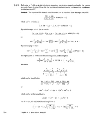
12. which gives the equations for the root-locus as follows:
w = o
The equation w = 0 represents the real axis. The root locus for 0 5 K 5 co is between points
s = -0.4 and s = -3.6. (The real axis other than this line segment and the origin s = 0 corre-
sponds to the root locus for -w 5 K < 0.)
The equations
represent the complex branches for 0 5 K 5 m.These two branches lie between a = -1.6 and
u = 0. [See Figure 6-44(b).] The slopes of the complex root-locus branches at the breakaway
point ( a = -1.2) can be found by evaluating d o l d a of Equation (6-21) at point a = -1.2.
Since tan-' a= 60°, the root-locus branches intersect the real axis with angles +60°
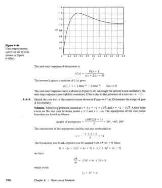
A-6-8. Consider the system shown in Figure 6-45(a), which has an unstable feedforward transfer func-
tion. Sketch the root-locus plot and locate the closed-loop poles. Show that, although the closed-
loop poles lie on the negative real axis and the system is not oscillatory,the unit-step response curve
will exhibit overshoot.
Solution. The root-locus plot for this system is shown in Figure 6-45(b).The closed-loop poles are
located at s = -2 and s = -5.
The closed-loop transfer function becomes
(a)
Figure 6-45
:a) Control system; (b) root-locus plot
Example Problems and Solutions
LClosed-loop zero

13. Figure 6-46
Unit-step response
curve for the system
shown in Figure
6-45 (a).
The unit-step response of this system is
The inverse Laplace transform of C ( s )gives
c(t) = 1 + 1.666~-~'- 2.666e-", fort 2 0
The unit-step response curve is shown in Figure 6-46.Although the system is not oscillatory, the
unit-step response curve exhibits overshoot. (This is due to the presence of a zero at s = -1.)
A-6-9. Sketch the root loci of the control system shown in Figure &47(a). Determine the range of gain
K for stability.
Solution. Open-loop poles are located at s = 1,s = -2 + j d , and s = -2 - j d . A root locus
exists on the real axis between points s = 1 and s = -03. The asymptotes of the root-locus
branches are found as follows:
*180°(2k + 1 )
Angles of asymptotes =
3
= 60°, -60°, 180"
The intersection of the asymptotes and the real axis is obtained as
The breakaway and break-in points can be located from dK/ds = 0. Since
K = -( r - l)(s2+ 4s + 7) = -(s3 + 3s2 + 3s - 7)
we have
which yields
(s + I ) ~= 0
Chapter 6 / Root-Locus Analysis

14. (a)
Figure 6-47
(a) Control system; (b) root-locus plot.
Thus the equation dK/ds = 0 has a double root at 3 = -1. (This means that the characteristic
equation has a triple root at s = -1.) The breakaway point is located at s = -1. Three root-locus
branches meet at this breakaway point.The angles of departure of the branches at the breakaway
point are ilX0°/3, that is. 60" and -60".
We shall next determine the points where root-locus branches may cross the imaginary axis.
Noting that the characteristic equation is
(.r - l)(.s2 + 4s + 7 ) + K = 0
or
.r+ 3 , ~ ~+ 3 . ~- 7 + K = o
we substitute s = jw into it and obtain
(jw)' + 3 ( j ~ ) ~+ 3(jw) - 7 + K -O
By rewriting this last equation, we have
( K - 7 - 3w2) + ,043 - w2) = 0
This equation is satisfied when
= K = 7 + 3 w " l 6 or w = 0 ,
Example Problems and Solutions

15. The root-locus branches cross the imaginary axis at w = h d (where K = 16)and w = 0 (where
K = 7). Since the value of gain K at the origin is 7, the range of gain value K for stability is
Figure 6-47(b) shows a sketch of the root loci for the system. Notice that all branches consist of
parts of straight lines.
The fact that the root-locus branches consist of straight lines can be verified as follows: Since
the angle condition is
we have
-1s - 1 - / s + 2 + j f l - /s + 2 - j d = h 1 8 0 ° ( 2 k + 1 )
By substituting s = a + jw into this last equation,
/u + 2 + j(w + d)+ / a + 2 + j(w - d)= - / a - 1 + jw f 180°(2k + 1 )
which can be rewritten as
w + a w - v 3
t a n ( ) + t ) = -tan-'(*) * L W ( 2 k + 1 )
Taking tangents of both sides of this last equation, we obtain
2w(u + 2 ) w
-
q 2 + 4 C T + 4 - w 2 + 3 a - 1
which can be simplified to
2w(u + 2 ) ( u - 1 ) = -w(a2 + 4 a + 7 - W 2 )
or
w(3a2 + 6 u + 3 - w2) = 0
Further simplification of this last equation yields
which defines three lines:
398 Chapter 6 / Root-i.o<cisAnalysis
C

16. Thus the root-locus branches consist of three lines. Note that the root loci for K > 0 consist of
portions of the straight lines as shown in Figure 6-47(b). (Note that each straight line starts from
an open-loop pole and extends to infinity in the direction of 180°,60°,or -60" measured from the
real axis.) The remaining portion of each straight line corresponds to K < 0.
A-6-10. Consider the system shown in Figure 6-48(a). Sketch the root loci
Solution. The open-loop zeros of the system are located at s = fj. The open-loop poles are lo-
cated at s = 0 and s = -2. This system involves two poles and two zeros. Hence, there is a possi-
bility that a circular root-locus branch exists. In fact, such a circular root locus exists in this case,
as shown in the following.The angle condition is
By substituting s = u + jw into this last equation, we obtain
Taking tangents of both sides of this equation and noting that
Figure 6-48
(a) Control system; (b) root-locus plot.
Example Problems and Solutions

17. we obtain
which is equivalent to
These two equations are equations for the root 1oci.Thefirst equation corresponds to the root locus
on the real axis. (The segment between s = 0 and s = -2 corresponds to the root locus for
0 5 K < m.The remaining parts of the real axis correspond to the root locus for K < 0.) The
second equation is an equation for a circle.Thus, there exists a circular root locus with center at
u = i,w = 0 and the radius equal to a / 2 . The root loci are sketched in Figure 6-48(b). [That
part of the circular locus to the left of the imaginary zeros corresponds to K > 0. The portion of
the circular locus not shown in Figure 6-48(b) corresponds to K < 0.1
A-6-11. Consider the control system shown in Figure 6-49. Plot the root loci with MATLAB.
Solution. MATLAB Program 6-11 generates a root-locus plot as shown in Figure 6-50.The root
loci must be symmetric about the real axis. However, Figure 6-50 shows otherwise.
MATLAB suppliesits own set of gain values that are used to calculate a root-locus plot. It does
so by an internal adaptive step-sizeroutine. However, in certain systems,very small changes in the
gain cause drasticchangesin root locationswithin a certain range of gains.Thus,MATLAB takes too
big ajump in itsgain values when calculatingthe roots,and root locationschange by a relatively large
amount.When plotting,MATLAB connects these points and causes a strange-looking graph at the
location of sensitive gains.Such erroneous root-locusplots typically occur when the loci approach a
double pole (or triple or higher pole),since the locus is very sensitive to small gain changes.
MATLAB Program 6-1 1
Figure 6 4 9
Control system.
num = [O 0 1 0.41;
den = [I 3.6 0 01;
rlocus(num,den);
v = [-5 1 -3 31; axis(v)
grid
title('Root-Locus Plot of G(s) = K(s + 0.4)/[sA2(s+ 3.6))')
Chapter 6 / Root-Locus Analysis

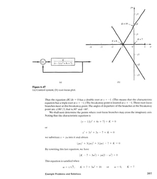
18. Figure (is0
Root-locus lot.
Root-Locus Plot of G(s) = K(s+0.4)/[s2(s+3.6)]
Real Axis
In the problem considered here, the critical region of gain K is between 4.2 and 4.4.Thus we
need to set the step size small enough in this region. We may divide the region for K as tollows:
Entering MATLAB Program 6-12 into the computer,we obrain the plot as shown in Figure 6-51,
If we change the plot command plot(r,'o')in MATLAB P r ~ g r a m6-12 to plot(r,'-'1,we obtain Fig-
ure 6-52. Figures 6-51 and 6-52 respectively, show satisfa~tc~ryroot-locus plots.
MATLAB Program 6-1 2
"A, -----.---- Root-locus plot ----------
num = [O 0 I 0.41;
den = [I 3.6 0 01;
K1 = [0:0.2:4.21;
K2 = [4.2:0.002:4.4];
K3 = [4.4:0.2:10];
K4 = [I 0:5:200];
K = [KI K2 K3 K4];
r = rlocus(num,den,K);
plot(r,'ol)
v = [-5 1 -5 51; axis(v)
grid
titIe('Root-Locus Plot of G(s) = K(s+ 0.4)/[sA2(s
xlabel('Rea1Axis')
ylabel('lmag Axis')
Example Problems and Solutions

19. Figure 6 5 1
Root-locus plot.
Figure 6 5 2
Root-locus plot.
Root-Locus Plot of G(s) = K(s+O 4)/[s2(s+3.6)]
5
0
-5 1 6
0
-5 -4 -3 -2 -1 0
Real AXIS
Root-Locus Plot of G(s)= K(s+0.4)/[s2(s+3.6)]
Real Axis
A-6-12. Consider the system whose open-loop transfer function G ( s ) H ( s )is given by
Using MATLAB,plot root loci and their asymptotes.
Solution. We shall plot the root loci and asymptotes on one diagram.Since the open-loop trans-
fer function is given by
G ( s ) H ( s )= -
K
s(s + l ) ( s + 2 )
-- K
s3 + 3s2 + 2s
the equation for the asymptotes may be obtained as follows:Noting that
lim
K
= lim
K K=-
3+m s3 + 3~~ + 2~ S-'m S~ + 3 ~ 2+ 3~ + 1 ( S + q3
Chapter 6 / Root-Locus Analysis

20. the equation for the asymptotes may be given by
num = [O O O 11
den = [I 3 2 01
and for the asymptotes,
numa = [O O O 11
dena = [I 3 3 11
In using the following root-locus and plot commands
the number of rows of r and that of a must be the same.To ensure this, we include the gain con-
stant K in the commands. For example,
MATLAB Program 6-1 3
num = [O O O I];
den = [I 3 2 01;
numa = [O 0 0 1I;
dena = [I 3 3 1I;
K1 = 0:0.1:0.3;
K2 = 0.3:0.005:0.5;
K3 = 0.5:0.5:10;
K4 = 1O:S:I 00;
K = [Kl K2 K3 K4];
r = rlocus(num,den,K);
a = rlocus(numa,dena,K);
y = [r a];
plot(y,'-'1
v = [-4 4 -4 41; axis(v)
grid
title('Root-LocusPlot of G(s)= K/[s(s+ 1)(s + 2)) and Asymptotes')
xlabel('Rea1Axis')
ylabeU1lmagAxis')
***** Manually draw open-loop poles in the hard copy *****
Example Problems and Solutions

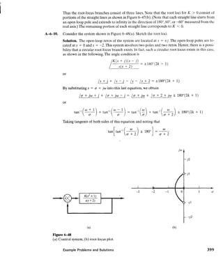
21. Root-Locus Plot of G(s) = Ki[(.s(s+l)(s+2)]and Asymptotes
Figure 6-53
Root-locus plot. Real Axis
Including gain K in rlocuscommand ensures that the r matrix and a matrix have the same number of
rows.MATLAB Program 6-13 will generate a plot of root loci and their asymptotes.SeeFigure6-53.
Drawing two or more plots in one diagram can also be accomplished by using the hold com-
mand. MATLAB Program 6-14 uses the hold command. The resulting root-locus plot is shown
in Figure 6-54.
MATLAB Program 6-1 4
01~------------ Root-Locus Plots ------------
num = [O 0 0 1I;
den = [ I 3 2 01;
numa = [O 0 0 11;
dena = (1 3 3 1I;
K1 = 0:0.1:0.3;
K2 = 0.3:O.OOS:O.S;
K3 = O.5:0.5:10;
K4 = 10:5:100;
K = [Kl K2 K3 K4];
r = rlocus(num,den,K);
a = rlocus(numa,dena,K);
plot(r,'ol)
hold
Current plot held
plot(a,'-'1
v = [-4 4 -4 41; axis(v)
grid
title('Root-Locus Plot of G(s) = K/[s(s+l )(s+2)1and Asymptotes')
xlabel('Rea1Axis')
ylabel('lmagAxis')
Chapter 6 / Root-Locus Analysis
.1

22. Root-Locus Plot of G(s) = Ki[.s(s+l)(s+2)]and Aysmptotes
Figure 6-54
Root-locus plot. Real Axis
Consider a unity-feedback system with the following feedforward transfer function G ( s ) :
K ( s + 2)'
C ( s ) = -
(s' + 4)(s + 5)'
Plot root loci for the system with MATLAB.
Solution. A MATLAB program to plot the root loci is given as MATLAB Program 6-15. The
resulting root-locus plot is shown in Figure 6-55.
Notice that this is a special case where no root locus exists on the real axis.This means that
for any value of K > 0 the closed-loop poles of the system are two sets of complex-conjugate
poles. (No real closed-loop poles exist.) For example, with K = 25, the characteristic equation
for the system becomes
s4 + 10s' + 54s' + 140s + 200
= (sL+ 4s + 10)(s2+ 6s + 20)
= (S + 2 + j2.4495)(s + 2 - j2.44!X)(s + 3 + ;3.3166)(s + 3 - j3.3166)
MATLAB Program 6-1 5
% ------------ Root-Locus Plot ------------
num = [O 0 1 4 41;
den = [I 10 29 40 1001;
r = rlocus(nurn,den);
plot(r,'ol)
hold
current plot held
plot(r,'-'1
v = [-8 4 -6 61; axis(v); axis('squarel)
grid
title('Root-Locus Plot of G(s) = (s + 2)"2/[(sA2 + 4)(s + 5)"211)
xlabel('Rea1Axis')
ylabel('lmag Axis')
Example Problems and Solutions

23. Root-Locus Plot of G(s)= ( ~ + 2 ) ~ / [ ( ~ ~ + 4 ) ( s + 5 ) * ]
Figure 6-55
Root-locus plot. Real Axis
Since no closed-loop poles exist in the right-half s plane, the system is stable for all values of
K > 0.
A-6-14. Consider a unity-feedback control system with the following feedforward transfer function:
Plot a root-locus diagram with MATLAB. Superimpose on the s plane constant 5 lines and con-
stant w , circles.
Solution. MATLAB Program 6-16 produces the desired plot as shown in Figure 6-56.
- - -
MATLAB Program 6-1 6
num = [0 0 1 21;
den = [I 9 8 01;
K = 0:0.2:200;
rlocus(num,den,K)
v = [ -10 2 -6 61; axis(v1; axis('squarel)
sgrid
title('Root-Locus Plot with Constant zeta Lines and Constant omega-n Circles')
gtext('zeta = 0.9')
gtext('0.7')
gtext('0.5')
gtext('0.3')
gtext('omega-n = 10')
gtext('8')
gtext('6')
gtext('4')
gtext('2')
Chapter 6 / Root-LocusAnalysis

24. Root-Locus Plot with Constant ( Lines and Constant onCircles
Figure 6-56
Root-locus plot with
constant 6 lilies and
constant w,, c:ircles. Real Axis
A-6-15. Consider a unity-feedback control system with the following feedforward transfer function:
Plot root loci for the system with MATLAB. Show that the system is stable for all values of K > 0.
Solution. MATLAB Program 6-17 gives a plot of root loci as shown in Figure 6-57. Since the root
loci are entirely in the left-half s plane, the system is stable for all K > 0.
MATLAB Program 6-1 7
num = [O 1 0 25 01;
den = [I 0 404 0 16001;
K = 0:0.4:1000;
rlocus(num,den,K)
v = [-30 20 -25 251; axis(v); axis('square')
grid
title('Root-Locus Plot of G(s) = K(sA2+ 25)s/(sA4+ 404sA2 + 1600)')
A-6-16. A simplified form of the open-loop transfer function of an airplane with an autopilot in the lon-
gitudinal mode is
Such a system involving an open-loop pole in the right-half s plane may be conditionally stable.
Sketch the root loci when a = b = 1, (' = 0.5, and w,, = 4. Find the range of gain K for stability.
Example Problems and Solutions 407

25. Root-Locus Plot of G(s) = ~ ( s ~+ 25)s/(s4+ 404s2+ 1600)
Figure 6-57
Root-locus plot. Real Axis
Solution. The open-loop transfer function for the system is
To sketch the root loci, we follow this procedure:
1. Locate the open-loop poles and zero in the complex plane. Root loci exist on the real axis
between 1and 0 and between -1 and -m.
2. Determine the asymptotes of the root loci.There are three asymptotes whose angles can be
determined as
180°(2k + 1)
Angles of asymptotes = = 60°,-60°, 180"
4 - 1
Referring to Equation (6-13), the abscissa of the intersection of the asymptotes and the real
axis is
3. Determine the breakaway and break-in points. Since the characteristic equation is
we obtain
By differentiating K with respect to s, we get
Chapter 6 / Root-Locus Analysis

26. The numerator can be factored as follows:
3s4 + 10s3 + 21s2 + 24s - 16
Points s = 0.45 and s = -2.26 are on root loci on the real axis. Hence, these points are actu-
al breakaway and break-in points, respectively. Points s = -0.76 f 12.16 do not satisfy the
angle condition. Hence, they are neither breakawav nor break-in points.
4. Using Routh's stability criterion, determine the value of K at which the root loci cross the
imaginary axis. Since the characteristic equation is
the Routh array becomes
The values of K that make the s' term in the first column equal zero are K = 35.7 and
K = 23.3.
The crossing points on the imaginary axis can be found by solving the auxiliary equation
obtained from the s2row, that is, by solving the following equation for s:
The results are
s = kj2.56, for K = 35.7
s = ij1.56, for K = 23.3
The crossing points on the imaginary axis are thus s = ~tj2.56and s = ij1.56.
5. Find the angles of departure of the root loci from the complex poles. For the open-loop pole
at s = -2 + j 2 d , the angle of departure 8 is
or
H = -54.5"
(The angle of departure from the open-loop pole at s = -2 - 12fl is 54S0.)
6. Choose a test point in the broad neighborhood of the jw axis and the origin, and apply the
angle condition. If the test point does not satisfy the angle condition, select another test point
until it does. Continue the same process and locate a sufficient number of points that satisfy
the angle condition.
Example Problems and Solutions 409

27. Figure 6-58
Root-locus plot.
Figure 6-58 shows the root loci for this system. From step 4, the system is stable for
23.3 < K < 35.7. Otherwise,it is unstable.Thus, the system is conditionally stable.
Consider the system shown in Figure 6-59, where the dead time T is 1sec. Suppose that we ap-
proximate the dead time by the second-order pade approximation. The expression for this ap-
proximation can be obtained with MATLAB as follows:
[num,den] = pade(1, 2);
printsys(num, den)
numlden =
s"2 - 6s + 12
Hence
Using this approximation, determine the critical value of K (where K > 0) for stability.
Solution. Since the characteristic equation for the system is
s + 1 + Ke-" = 0
Chapter 6 / Root-LocusAnalysis

28. Figure 6-59
A control system
with dead time.
by substituting Equation (6-22) into this characteristic equation, we obtain
Applying the Routh stability criterion, we get the Routh table as follows:
Hence, for stability we require
-6K2 - 36K + 114 > 0
which can be written as
(K + 8.2915)(K - 2.2915) < 0
or
K < 2.2915
Since K must be positive, the range of K for stability is
0 < K < 2.2915
Notice that according to the present analysis, the upper limit of K for stability is 2.2915.This
value is greater than the exact upper limit of K. (Earlier, we obtained the exact upper limit of K
to be 2, as shown in Figure 6-38.) This is because we approximated e-" by the second-order pade
approximation.A higher-order pade approximation will improve the accuracy. However, the com-
putations involved increase considerably.
A-6-18. Consider the system shown in Figure 6-60.The plant involves the dead time of T sec.Design a suit-
able controller G,(s) for the system.
Solution. We shall present the Smith predictor approach to design a controller.The first step to
design the controller G,(s) is to design a suitable controller G,(s) when the system has no dead
time. Otto J.M. Smith designed an innovative controller scheme, now called the "Smith predictor,"
Example Problems and Solutions 411

30. Then the closed-loop transfer function C(s)/R(s)can be given by
Figure 6-62
Step-response
curves.
Hence,the block diagram of Figure 6-61(a) can be modified to that of Figure 6-61(b).The closed-
loop response of the system with dead time e-TJisthe same as the response of the system with-
out dead time c-~',except that the response is delayed by T sec.
Typical step-response curves of the system without dead time controlled by the controller
&,(s) and of the system with dead time controlled by the Smith predictor type controller are
shown in Figure 6-62.
It is noted that implementing the Smith predictor in digital form is not difficult,because dead
time can be handled easily in digital control. However, implementing the Smith predictor in an
analog form creates some difficulty.
Step Response
Sm~thpredictor type controller
1
0 0.5 1 1.5 2 2.5 3 3.5 4 4.5 5
Time (sec)
PROBLEMS
B-6-1. Plot the root loci for the closed-loopcontrol system B-6-3. Plot the root loci for the closed-loop control system
with with
. .
B-6-2. Plot the root loci for the closed-loop control system
with B-6-4. Plot the root loci for the system with
Problems 413

31. B-6-5. Plot the root loci for a system with
Determine the exact points where the root loci cross the jw
axis.
8-64. Show that the root loci for a control system with
are arcs of the circle centered at the origin with radius equal
to m.
8-6-7. Plot the root loci for a closed-loop control system
with
B-6-8. Plot the root loci for a closed-loop control system
with
B-6-9. Plot the root loci for a closed-loop control system
with
Locate the closed-loop poles on the root loci such that the
dominant closed-loop poles have a damping ratio equal to
0.5.Determine the corresponding value of gain K.
B-6-10. Plot the root loci for the system shown in Figure
6-63. Determine the range of gain K for stability.
Figure 6-63
Control system.
R-6-11. Consider a unity-feedback control system with the
following feedforward transfer function:
Plot the root loci for the system. If the value of gain K is set
equal to 2,where are the closed-loop poles located?
B-6-12. Consider the system whose open-loop transfer
function G(s)H(s)is given by
Plot a root-locus diagram with MATLAB.
B-6-13. Consider the system whose open-loop transfer
function is given by
Show that the equation for the asymptotes is given by
Using MATLAB, plot the root loci and asymptotes for
the svstem.
B-6-14. Consider the unity-feedback system whose feed-
forward transfer function is
The constant-gain locus for the system for a given value of
K is defined by the following equation:
Show that the constant-gain loci for 0 5 K 5 comay be
given by
Sketch the constant-gain loci for K = 1,2,5,10,and 20 on
the s plane.
B-6-15. Consider the system shown in Figure 6-64. Plot the
root loci with MATLAB.Locate the closed-loop poles when
the gain K is set equal to 2.
u
Figure 6-64
Control system.
414 Chapter 6 / Root-Locus Analysis

32. B-6-16. Plot root-locus diagrams for the nonminimum- B-6-17. Consider the closed-loop system with transport lag
phase systemsshown in Figures6-65(a) and (b),respectively. shown in Figure 6-66. Determine the stability range for
gain K.
Figure 6-66
Control system.
Figure 4-65
(a) and (b) Nonminimum-phase systems.
Problems