This document summarizes the numerical solution of the time-independent Schrodinger equation for particles in chaotic stadium and Sinai billiard potentials using the finite difference method. Scars, or regions of high probability density around unstable periodic orbits, were observed in particular eigenstates of both systems, consistent with previous studies. The method was validated by reproducing analytical solutions for 1D and circular wells and showing convergence of eigenvalues with increasing numerical resolution.

1. Scars in the Wavefunction of the Stadium
Billiard
Paolo Pichini, Nathan Simpson
9438499, 9440203
School of Physics and Astronomy
The University of Manchester
2nd Year Theory Computing Project
May 2016
Abstract
The time independent Schr¨odinger equation was solved numerically using the method
of finite differences for two classically chaotic systems: a stadium-shaped potential well
and a rectangular well with a circular region of infinite potential at its centre, better known
as Sinai billiard. In both cases “scars” - defined as regions of high probability density
surrounding an unstable periodic orbit - were observed for particular states, confirming
previous studies.

2. 1 Introduction
The particle in a one-dimensional infinite potential well is a problem that is well under-
stood in quantum physics. By solving the time independent Schr¨odinger equation (TISE),
we can obtain the wavefunctions corresponding to each value of the quantum number,
and henceforth for each allowed value of the energy. We can extend this problem to two
dimensions fairly easily in the case of a square or a rectangle.
However, not all shapes of potential well can be solved analytically. Of these cases,
this report will focus primarily on the case of the stadium-shaped well, which is defined
as a square with semicircular wells affixed to either end and it is a classically chaotic
system (see Fig. 1). The reason for this is that it is known that “scars” - defined as
regions of high probability density surrounding an unstable periodic orbit - are observed
in particular wavefunctions of the stadium problem [1]. These “scars” can be explained
by the Ehrenfest theorem, which shows that quantum mechanical expectation values obey
Newton’s equations of motion, although it should be noted that this statement has some
caveats [2].
This investigation aims to recover the scars seen in the pioneering studies by McDonald
[3][4] by solving the TISE numerically using the method of finite differences. Mathemat-
ica is the only software used throughout this investigation. Another well-known chaotic
system that produces scars - the Sinai billiard (see Fig. 1) - will also be investigated in the
same manner.
Figure 1: A diagram showing a stadium billiard on the left and a Sinai billiard on the right. Note
that the proportions of the Sinai billiard can vary.
2 Theory and Numerical Method
1D well
The potential of a particle trapped inside a 1D infinite well is:
V(x) =
0 if 0 ≤ x ≤ L,
∞ otherwise.
(1)
The wavefunction must be zero where the potential is infinite. Instead, within the region
of zero potential, which we will refer to as “the well”, the TISE can be written as:
∂2ψ
∂x2
= −
2mE
¯h2
ψ (2)
1

3. where m is the particle’s mass and ψ is the wavefunction in position space. This equation
has well known analytical solutions:
ψ(x) =
2
L
sin(
nπx
L
) (3)
n = 1,2,3,...
The first step of our analysis was to reproduce such solutions using numerical methods,
which are described below. The well can be modelled as a set of discrete points separated
by equal intervals, with ψ taking a value ψi at the ith point. Hence, if there are m points,
the distance between each point (the “stepsize”) will be δL = L
m−1. Now, consider the
following expansions:
ψi+1 = ψi +δL
∂ψ
∂x
+
δL2
2
∂2ψ
∂x2
+
δL3
6
∂3ψ
∂x3
+O(δL4
), (4)
ψi−1 = ψi −δL
∂ψ
∂x
+
δL2
2
∂2ψ
∂x2
−
δL3
6
∂3ψ
∂x3
+O(δL4
). (5)
Adding (4) and (5) together and rearranging, we obtain:
ψi−1 −2ψi +ψi+1
δL2
=
∂2ψ
∂x2
+O(δL2
). (6)
It can be observed that the second derivative is approximately equal to the LHS, where
the error is proportional to the square of the stepsize. Hence, if δL 1, we can combine
(2) and (6) to obtain:



−ψi−1 +2ψi −ψi+1 = λψi,
λ = 2mEδL2
¯h2
. (7)
This is known as the finite differences method, and it yields a system of m linear equations
(one for each point on the well) that can be written in matrix form:







2 −1 ··· ··· 0
−1 2 −1 ··· 0
0
...
...
...
...
...
0 ··· −1 2 −1
0 ··· ··· −1 2







×







ψ1
ψ2
ψ3
...
ψm







= λ ×







ψ1
ψ2
ψ3
...
ψm







, (8)
where all entries on the main diagonal are “2”, all those on the superdiagonal and subdi-
agonal are “-1” and all other entries are zero. This is an eigenvalue problem and can be
solved numerically. Each eigenvector encodes within it the value of the wavefunction at
all points in the well for one particular eigenstate.
2

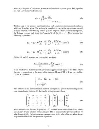
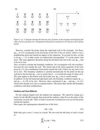
4. 2D rectangular well
A 2D rectangular well is a rectangular region of zero potential surrounded by a region of
infinite potential. Similarly to the 1D case, the well can be discretised to an array of points
(see Fig 2(a)). Each point can be labelled by the coordinates (i,j), where i and j represent
the number of “steps” away from the top-left corner in the x (horizontal) and y (vertical)
directions respectively. We require the stepsize to be the same in both directions, as this
will be necessary to solve the problem. For convenience, we will use the term “rows” to
refer to the sets of points with fixed j, and “columns” for those with fixed i. The TISE is
now:
∂2ψ
∂x2
+
∂2ψ
∂y2
= −
2mE
¯h2
ψ (9)
As before, we can approximate each of the derivatives at a point (i,j) using the method of
finite differences (see equation (6)). For the y derivative, the points considered will be the
neighbouring points of (i,j) in the same column, whereas they will be those in the same
row for the x derivative (see Fig. 2(b)). By substituting the results in (9), we obtain:
−ψi,j−1 −ψi−1,j +4ψi,j −ψi+1,j −ψi,j+1 = λψi,j, (10)
where λ = 2mEδL2
¯h2 as before. If the rectangle has sides Lx and Ly, to take equal steps in
each direction, we must define our stepsize as
δL =
Lx
n−1
=
Ly
m−1
,
where n is the number of points in one row of the well and m is the number of points in
one column.
Then, to simplify the problem, each point on the rectangle can be labelled with a single
number - α, say - rather than with a pair of coordinates. To make this possible, a mapping
is necessary of the form (i,j) → α. We deduced that an appropriate mapping would be to
label the first row of points of the well from 1 to n, the second row as n+1 to 2n and so on
(see example in Fig 2(a), for a 5δLx3δL rectangle).
Since i ∈ [0,n−1] and j ∈ [0,m−1] the mapping can be expressed as α = i+nj +1. As
a result, α ∈ [1,mn]. Therefore, equation (10) can be rewritten in terms of α:
−ψα−n −ψα−1 +4ψα −ψα+1 −ψα+n = λψα. (11)
As before, this results in a set of linear equations that can be written in matrix form to
obtain an eigenequation. In this case, the eigenvectors will contain entries ψα for each
point on the rectangle and the matrix will be a mn x mn square matrix.
3

5. Figure 2: (a): A diagram showing the discrete array of points on the rectangle and displaying the
value of α for each point; (b): Arrangement of the points considered in (10), known as the 5-points
stencil.
However, consider the points along the right-hand wall of the rectangle. For those,
ψα+1 in (11) corresponds to the first point on the left in the row below, which is not a
neighbouring point and should not appear in the expansion. To account for this, we had
to set ψα+1 = 0: in other words, we replaced the correspondent “-1”s in the matrix with
zeros. The same applied to the points along the left-hand wall, but in this case ψα−1 had
to be set to zero.
Also, we had to consider the boundary conditions: for a rectangular well, the wavefunc-
tion must be zero outside the well. This means that in the linear equations of the form
given by (11), the contributions from points outside the well, if there are any, have to be
set to zero. This boundary condition is satisfied automatically for the points on the top
wall due to the fact that ψα−n has to vanish, but α −n is outside the range of values of α.
The same applies to the bottom well, but in that case, ψα+n has to vanish instead.
In addition, for the left-hand and right-hand walls, the boundary conditions require ψi−1,j
and ψi+1,j in (10) to be zero. However, these correspond to ψα−1 and ψα+1 in (11),
which were already set to zero as explained above. The matrix then satisfies the boundary
conditions with these modifications.
Stadium and Sinai Billiards
For the stadium-shaped well, the method was analogous. We started by setting up a
matrix for the 4Rx2R rectangle that enclosed the stadium, where R was the radius of the
semicircles on each side. Then, we had to ensure the wavefunction was zero for the points
outside the stadium.
Once again, the eigenequation obtained was of the form:
Aψ = λψ. (12)
Both sides give a mn x 1 vector as a result. We can write the αth entry of such a vector
as:
mn
∑
k=1
Aα,kψk = λψα. (13)
4

6. Note that ψα corresponds to the value of the eigenfunction at the point α. Hence, if
the point was outside the stadium, we needed to set ψα = 0. Assuming λ = 0, this is
equivalent to both sides of (13) being zero. This was achieved by setting Aα,k = 0 for all
k, in other words by replacing the αth row of A with a row of zeros. However, this allowed
for additional solutions with a zero eigenvalue. We identified these as flawed solutions
and removed them from the results. The rows that corresponded to points inside the
stadium, instead, remained unchanged, and the new boundary conditions were satisfied
by us requiring the wavefunction to be zero outside the stadium.
The same method was used for a circular well to test if it produced valid solutions in
comparison with the analytical solutions. In fact, we found a good agreement between
the two, as shown in Fig. 3.
Figure 3: A colour plot of the probability amplitude for the 7th excited state of a free particle
in a circular well, calculated both numerically (left) and analytically (right). The accurate corre-
spondence was verified for all states considered and it validates the method used for the boundary
conditions.
The case of the Sinai billiard was also explored. The shape of the well in this case is
a rectangle with a circular region of infinite potential, or “pillar”, in the centre. For our
analysis, we decided to use a 20x10 rectangle and a pillar of radius 1 (arbitrary units).
The method to set up the matrix was identical to the stadium, but different points were
removed since the shape was different.
3 Results and Discussion
For the 1D case, we obtained numerically the eigenvectors and eigenvalues and ob-
served a good correspondence with their analytical counterpart. Fig. 4(a) displays a plot
of the eigenvalues obtained via both methods: we can see that the numerical approxima-
tion diverges significantly from the exact result after about a third of the eigenvalues.
A similar test was performed for the 2D rectangular well. In this case, as shown in Fig.
4(b), the two curves diverged significantly after about a sixth of the eigenvalues, resulting
in a smaller fraction of reliable results than in the 1D case.
5

7. Figure 4: A graph of the numerical eigenvalues (blue) and the analytical eigenvalues (orange)
plotted against state number for the one-dimensional well (a) and a rectangular well (b). The
number of points on the well was 150 in the 1D case, 19900 in the rectangular case.
6

8. From (6), we can see that by reducing the stepsize we reduce the error on the approxi-
mation. Therefore, increasing the number of points (mn) on the rectangle is equivalent to
improving the reliability of the solutions. This is shown in Fig. 5 by comparison with the
analytical solutions for the case of a 4Rx2R rectangle, where R is an arbitrary constant.
Note that since the dimensions are fixed, defining m suffices to define the total number
of points and therefore the resolution. Since both the stadium and the Sinai billiards are
enclosed in a 4Rx2R rectangle in our analysis, m will also be quoted for these cases.
Figure 5: Fractional error of the eigenvalues for the rectangle, for m = 50 (b) and m = 100 (a).
In the stadium case, the accuracy could not be measured by comparison with the analytical
solution due to a lack thereof. We therefore assumed the same number of solutions would
be reliable as in the case of a 4Rx2R rectangle, since the approximation found via the finite
differences method was of the same form for both problems (see (11)). In the rectangular
case, a result was considered reliable if its corresponding eigenvalue was different from
its analytical counterpart by less than 5%. For example, as shown in Fig. 5, the first 300
eigenfunctions and values approximately were found to be reliable for m = 100.
Another method to check the accuracy was to compare results for different resolutions.
Fig. 6(a) plots the first 130 eigenvalues for different values of m: we can see that the
curves get closer as m increases, hence it is reasonable to assume such values are reliable
for m = 80 or higher. To confirm this, Fig. 6(b) shows that the fractional difference
between the same eigenvalues for m = 80 and m = 100 is less than 1.5% for all states
considered in our analysis. Similar findings were obtained for the Sinai billiard and are
presented in Fig. 6(c) and 6(d). The results presented in this report were all obtained
for m = 100 and are within the first 130 states, hence they can be considered reliable by
the previous arguments. Such results, for both the stadium and the Sinai billiards, are
presented in the next subsections.
Stadium Billiard
The letter ‘k’ will be used hereon to label the kth state (and wavefunction) from the
lowest energy state to higher states. The following plots depict the probability density
for a free quantum particle in the stadium in the kth energy state. It is worth noting that
the numbers shown by the legend are not normalised and are only significant as a relative
measure of probability. The axes of the plots define the particle’s horizontal and vertical
position in the well in arbitrary units: in fact, they form the sides of the 4Rx2R rectangle
enclosing the stadium/pillar.
7

9. Figure 6: (a): Superposed eigenvalue plots for different values of m; (b): Fractional difference
between numerical eigenvalues for m = 80, 100. (c), (d): Same as (a) and (b) but for the Sinai
billiard. It must be noted that λ depends on the stepsize and hence on m, as shown in (7). Hence,
to compare the results at different resolutions, we must plot λ
δL2 .
The first scar in the wavefunctions of the stadium was observed for k = 68, shown in
Fig. 7(a). In this case, the classical orbit passes through the centre of the stadium (i.e. the
centre of the central square) and traces two equilateral triangles.
Another scar was observed for k = 108 and is displayed by Fig. 7(b). The trajectory
corresponds to a particle bouncing back and forth between the top and bottom walls of
the stadium. It is interesting to note that three independent orbits are displayed in the same
plot, one for each vertical line. However, the concept of a particle confined to a single,
well defined orbit is only meaningful within the framework of classical mechanics. In
quantum mechanics, instead, scars tracing multiple orbits still satisfy the predictions of
the Ehrenfest theorem and hence are in no way different from scars mapping to a single
orbit.
Another case was found for k = 87 (Fig. 7(c)). Here the orbit traces a rectangle and
it intersects the circular wells at an angle of 45 degrees with respect to the horizontal,
calculated from the centre of curvature of the semicircles.
Finally, we present the scars observed for k = 127 (Fig. 7(d)). At first glance, it would
seem that this state does not map to any regular classical orbit. On the other hand, the
diamond-shaped orbit reproduced by the red line in the figure (not there yet) does cross
all regions of highest probability in the plot. It remains unclear whether states like these
(of which there are many) correspond to clearly defined classical orbits.
8

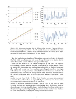
10. Figure 7: Density plot of the probability distribution for k = 68 (a), 108 (b), 87 (c), 127 (d).
The green lines represent the correspondent classical orbits. The different colours on the plots
correspond to a different probability density and a relative measure is provided by the legends.
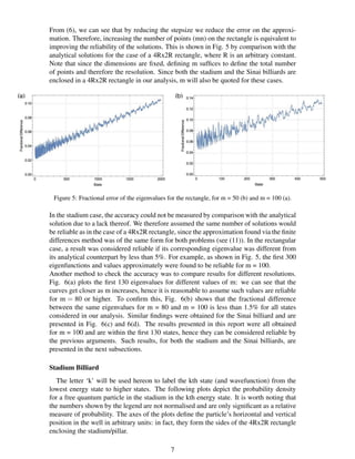
Sinai Billiard
A wide range of scars was found for the case of a Sinai billiard. In this report, only the
most significant one will be presented. This was found for k = 98, as shown in Fig. 8.
In this case, the scars trace an orbit that, classically, would be allowed in the case of a sim-
ple 20x10 rectangle, without a central pillar. Although, no scars appear in the rectangular
case, which has simple sinusoidal solutions. On one hand, this confirms the different view
of reality provided by quantum mechanics: the presence of the pillar would only influ-
ence a classical particle if its orbit comes to contact with it, whereas it always influences
a quantum state, which depends on the form of the potential for the entire space. On the
other hand, it confirms that scars do not arise in simple non-chaotic systems, with some
exceptions [5]. Instead, they appear for classically chaotic systems with a few periodic
orbits, and those systems are usually the object of scar-related scientific studies [6].
9

11. Figure 8: This image displays a density plot of the probability distribution for the 98th quantum
state. The green line represents the correspondent classical orbit. The colours correspond to
a different probability, as shown by the legend. Note that the central circle (of radius 1) is a
forbidden region in the case of the Sinai billiard.
4 Conclusion
We have successfully managed to solve the problem of a particle trapped in a stadium-
shaped potential well numerically. Moreover, we have confidence in our method from the
fact that we recovered several well-known scars that correspond to classical orbits of a
billiard. The same was able to be done for the Sinai billiard.
One of the major limitations of this project was that we were unable to assign an error
to the stadium eigenvalues due to a lack of analytical results to compare with, so we de-
cided to take the tolerance limit from the rectangular well. This could be amended by
approximately solving the TISE for an arbitrarily-shaped potential well analytically using
a method created by Kaufman, Kosztin and Schulten known as the expansion method [7].
This pseudo-analytic method would provide another way to assign an error to the eigen-
values and eigenvectors found numerically for the stadium and Sinai billiard by means of
an appropriate comparison.
Another limitation on the project was that our equipment limited the maximum value of m
we could use. A computer with significantly higher processing speed would allow many
more eigenvalues to be within the 5% tolerance limit and hence extend the scope of our
analysis to much higher energies, along with improving the accuracy of the eigenvalues
and the distinctness of the scars in the process.
Additionally, we could have produced the wavefunctions by only considering the upper
quarter of the stadium and reflecting it so it filled up the whole stadium. This way, the
size of the matrix would have been reduced to a quarter and the calculations would have
been faster. However, such a method would only allow to explore cases with a certain
symmetry with respect to the axes that divide the stadium in four sections. On the other
hand, it would produce reliable results for higher energy states at accessible resolutions,
since these stases would be found faster, being part of the reduced set of symmetric cases.
Taking this project further would involve investigating a wide variety of shapes to try and
find scarred wavefunctions for these cases. The case of a three-dimensional stadium, or
“pill”, could also be investigated to see if scars could be found in three dimensions.
10

12. References
[1] E. J. Heller. Bound-State Eigenfunctions of Classically Chaotic Hamiltonian Sys-
tems: Scars of Periodic Orbits. Phys. Rev. Lett. 1984; 53(16): 1515-1518.
[2] Nicholas Wheeler. Remarks concerning the status and some ramifications of Ehren-
fest’s Theorem. Reed College Physics Department. 1998.
Available from: http://www.reed.edu/physics/faculty/wheeler/documents/Quantum%20
Mechanics/Miscellaneous%20Essays/Ehrenfest’s%20Theorem.pdf [Accessed 27th
April 2016].
[3] S. W. McDonald. Lawrence Berkeley Laboratory. Report number: LBL-14837,
1983 (unpublished).
[4] S. W. McDonald and A. N. Kaufman. Phys. Rev. Lett. 1979; 42(1189).
[5] P. Seba, K. Zyczkowski. Wave Chaos in Quantized Classically Nonchaotic Sys-
tems. Physical Review A. 1991; 44(6).
[6] T. M. Antonsen et al. Statistics of Wave-Function Scars. Physical Review E. 1995;
51(1).
[7] D. L. Kaufman, I. Kosztin and K. Schulten. Expansion method for stationary states
of quantum billiards. Am. J. Phys. 1998; 67(1): 133-141.
11