The document discusses design of control systems using root locus analysis and compensation techniques. It provides examples of using lead and lag compensation to improve transient response and steady state error, respectively. The key steps are:
1) Analyze the uncompensated system root locus
2) Translate design specifications to a desired closed loop pole location
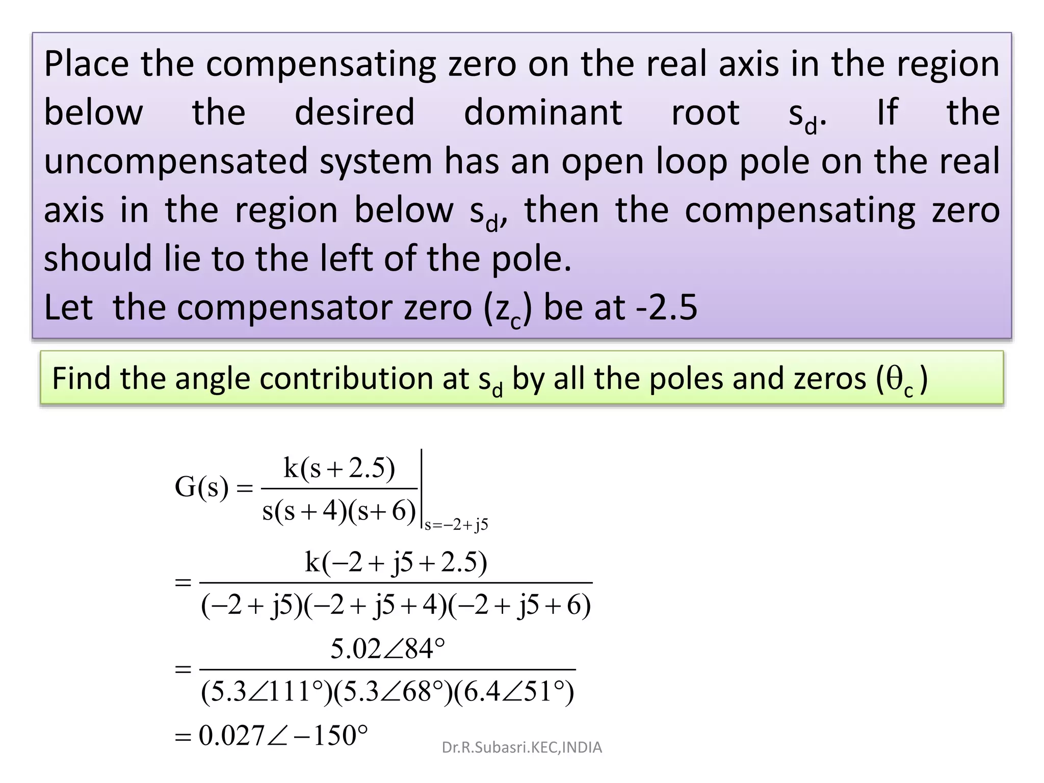
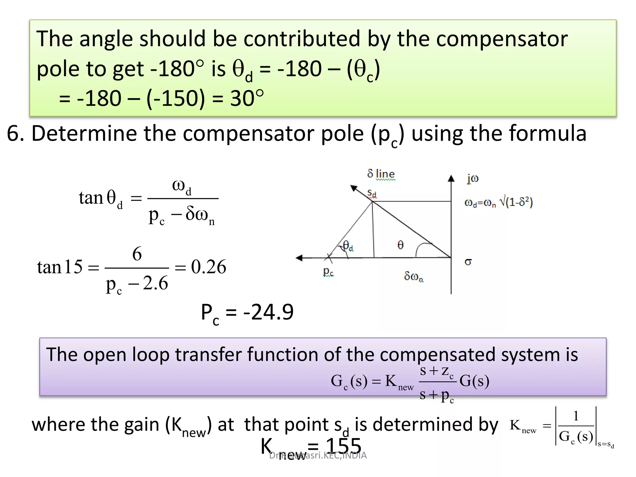
3) Determine compensator pole and zero locations to shape the root locus through the desired pole
4) Calculate the new open loop transfer function and gain to achieve the design specifications