This document introduces the root locus technique for analyzing how the closed-loop poles of a control system vary with changes in the controller gain. It provides 5 rules for constructing a root locus diagram:
1) Locate open-loop poles and zeros.
2) The number of root locus branches equals the greater of open-loop poles or zeros.
3) Points on the real axis are on the locus if open-loop poles/zeros to the right are odd.
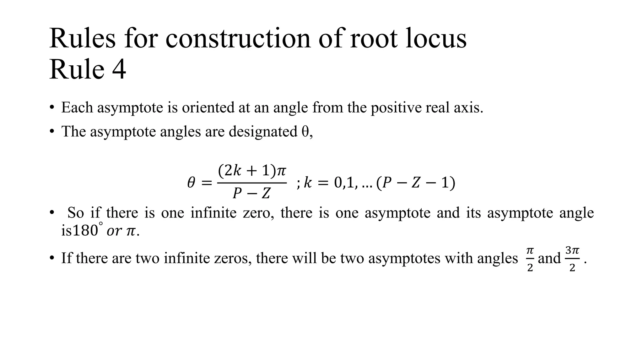
4) Asymptotes radiate from the centroid at fixed angles depending on open-loop poles/zeros.
5) Branches depart breakaway points where multiple roots occur at angles of ±180/n degrees.