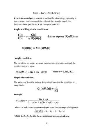
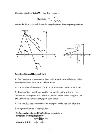
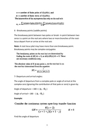
1. Root locus analysis graphically displays the location of closed-loop poles as a function of the open-loop gain K. 2. Root loci start at open-loop poles when K=0 and end at open-loop zeros or infinity as K approaches infinity. There are an equal number of loci and system order. 3. Breakaway points occur where loci depart or arrive at the real axis between poles or zeros. These may be complex.

1. 1
Root – Locus Technique
A root- locus analysis is analytical method for displaying graphically in
the s- plane , the location of the poles of the closed – loop T.F as
function of the gain factor K of the open- loop T.F
Angle and Magnitude conditions:
Angle condition:
The condition on angles are used to determine the trajectories of the
root loci in the s- plane
Magnitude condition:
The values of K on the loci are determined by using the condition on
magnitude .
Example:

2. 2
Construction of the root loci:
1 - Each locus starts at an open- loop pole when k = 0 and finishes either
at an open – loop zero or ∞ , when k = ∞
2 - The number of branches of the root loci is equal to the order system
3 - Points of the root –locus on the real axis lie to the left of an odd
number of finite poles and zeros for k>0.Loci either move along the real
axis or occur as complex conjugate pairs of loci
4 - The root loci are symmetrical with respect to the real axis of plane
5 – Angle and center of asymptotes:

3. 3
6 - Breakaway points (saddle points)
The breakaway point between two poles or break -in point between two
zeros is a point on the real axis where two or more branches of the root-
locus depart from or arrive at the real axis
Note: A root locus plot may have more than one breakaway point.
Breakaway points may be complex conjugates
7- Departure and arrival angles:
The angle of departure from a complex pole or angle of arrival at the
complex zero (ignoring the contribution of that pole or zero) is given by
Angle of departure = 180 + ( ɸz - Өp )
Angle of arrival = 180 - ( ɸz - Өp )
Example:
Find the angle of departure

4. 4
Solution: 180 + (45 – 90) = 135
8 – Intersection of the root loci with the imaginary axis and calculation of
k and frequency of oscillation ω
The limiting value of k for stability may be found using the routh array
on the characteristic equation
Example: Consider the system shown in figure below . Sketch the root –
locus plot and then determine the value of k such that the damping
ratio of a pair of dominant poles is 0.5
Solution:
The open – loop T.F G(s) H(s) =
Number of open – loop poles n= 3
Number of open – loop zeros m=0
3rd
order system, The number of loci (branches) = n =3
number of asymptotes = n-m = 3-0=3
The number of asymptotes angles = n -m =3-0=3

5. 5
Angle and center of asymptotes:
i = 0 , 1 , 2 : Ө0 = 60 , Ө1 = 180 , Ө2 = 300 = - 60
Center of asymptotes = ( - 1 -2 ) - 0 / (3 - 0) = - 1
Breakaway points : The characteristic equation is:
K = S3
+ 3S2
+ 2S
dK / dS = 3S2
+6S +2 = 0 notes s= -1.5774 neglected

6. 6
The crossing points on the imaginary axis
The characteristic equation is:
The routh array becomes
The value of K at breakaway points s = - 0.4226 is 0.384
0<K<0.384 overdamped , K =0.384 critical damped , 0.384<K<6 underdamped
K = 6 critical stable , K > 6 unstable system

7. 7
Example :Consider the control system shown in figure below. Sketch the
root – locus plot and determine the approximate damping ratio for a
value of K = 1.33
Solution:
n=2 , m = 1 , 2nd
order system , 2 loci , 1 asymptotes , 1 angle ,Ө0=180
The angle of departure is

8. 8
The characteristic equation is:
S2
+ ( 2 + K ) S + 3 + 2K = 0 , for K = 1.33
S2
+ 3.33 S + 5.66 = 0 , S1 = - 1.665 + J 1.699 , ω = 1.699 , α =1.665
ө = tan -1
= ω/ α = 450
, ζ =0.707
Example: Sketch the root – locus plot for the system shown in figure below
Solution:

9. 9

10. 10

11. 11
Example: Sketch the root locus for the system shown in fig below.
Solution:
Center of asymptotes
Angles of asymptotes = 60 , 180 , 300
The closed-loop T.F
For stability 90-k>0, 21k>0 -k2
-65k+720 / 90-k >0
From equation
dk/ds=3s4
+26s3
+77s2
+84s+24 breakaway point =-0.43
( 90-9.65)s2
+21(9.65)= 0 ω=1.59 rad/sec