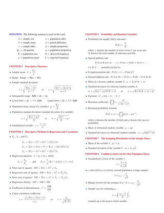
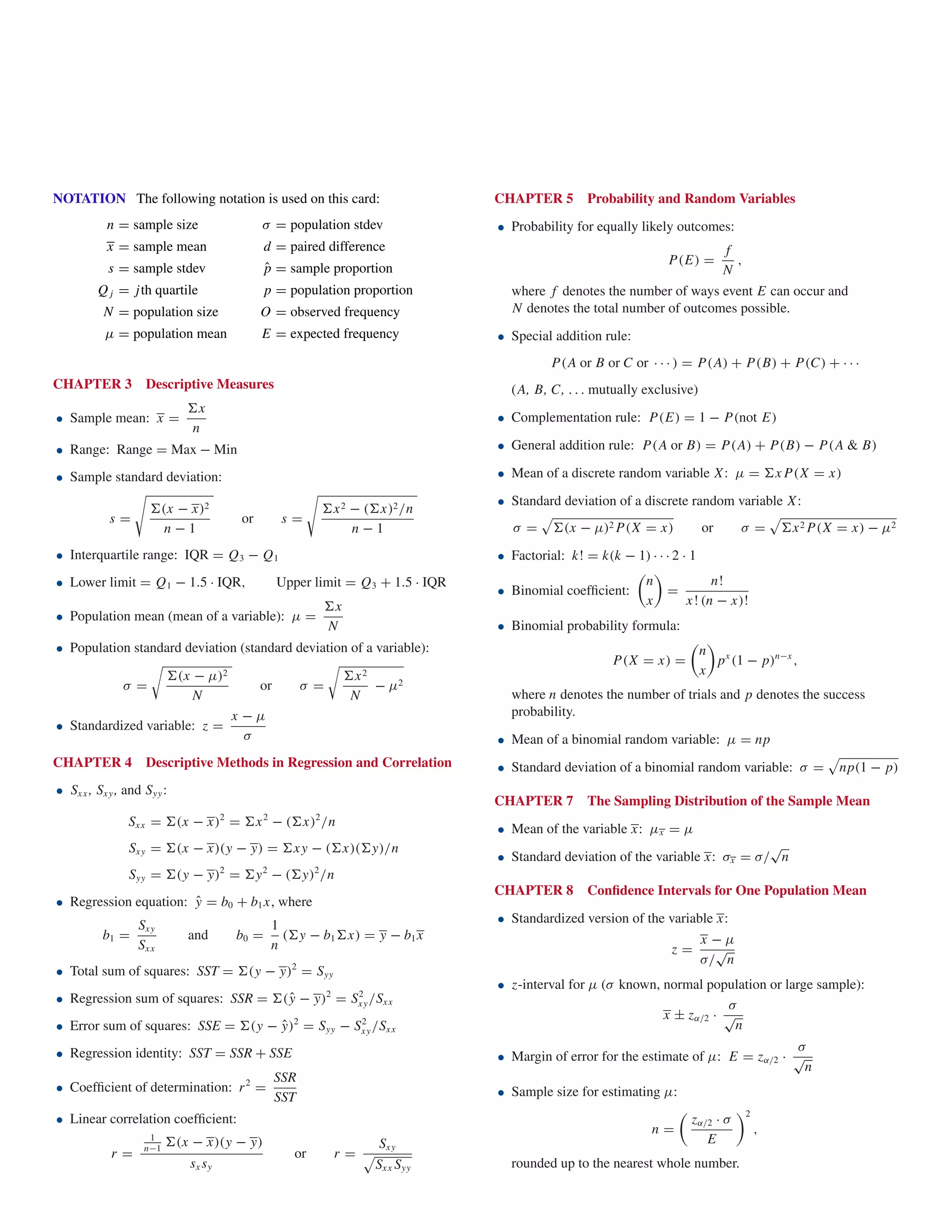
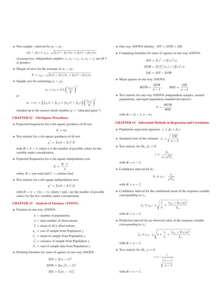
NOTATION The following notation is used on this card:
n sample size
x sample mean
s sample stdev
Qj jth quartile
N population size
µ population mean
σ population stdev
d paired difference
ˆp sample proportion
p population proportion
O observed frequency
E expected frequency
CHAPTER 3 Descriptive Measures
• Sample mean: x
x
n
• Range: Range Max − Min
• Sample standard deviation:
s
(x − x)2
n − 1
or s
x2 − ( x)2/n
n − 1
• Interquartile range: IQR Q3 − Q1
• Lower limit Q1 − 1.5 · IQR, Upper limit Q3 + 1.5 · IQR
• Population mean (mean of a variable): µ
x
N
• Population standard deviation (standard deviation of a variable):
σ
(x − µ)2
N
or σ
x2
N
− µ2
• Standardized variable: z
x − µ
σ
CHAPTER 4 Descriptive Methods in Regression and Correlation
• Sxx, Sxy, and Syy:
Sxx (x − x)2
x2
− ( x)2
/n
Sxy (x − x)(y − y) xy − ( x)( y)/n
Syy (y − y)2
y2
− ( y)2
/n
• Regression equation: ˆy b0 + b1x, where
b1
Sxy
Sxx
and b0
1
n
( y − b1 x) y − b1x
• Total sum of squares: SST (y − y)2
Syy
• Regression sum of squares: SSR (ˆy − y)2
S2
xy/Sxx
• Error sum of squares: SSE (y − ˆy)2
Syy − S2
xy/Sxx
• Regression identity: SST SSR + SSE
• Coefficient of determination: r2 SSR
SST
• Linear correlation coefficient:
r
1
n−1
(x − x)(y − y)
sxsy
or r
Sxy
SxxSyy
CHAPTER 5 Probability and Random Variables
• Probability for equally likely outcomes:
P(E)
f
N
,
where f denotes the number of ways event E can occur and
N denotes the total number of outcomes possible.
• Special addition rule:
P(A or B or C or · · · ) P(A) + P(B) + P(C) + · · ·
(A, B, C, . . . mutually exclusive)
• Complementation rule: P(E) 1 − P(not E)
• General addition rule: P(A or B) P(A) + P(B) − P(A & B)
• Mean of a discrete random variable X: µ xP(X x)
• Standard deviation of a discrete random variable X:
σ (x − µ)2P(X x) or σ x2P(X x) − µ2
• Factorial: k! k(k − 1) · · · 2 · 1
• Binomial coefficient:
n
x
n!
x! (n − x)!
• Binomial probability formula:
P(X x)
n
x
px
(1 − p)n−x
,
where n denotes the number of trials and p denotes the success
probability.
• Mean of a binomial random variable: µ np
• Standard deviation of a binomial random variable: σ np(1 − p)
CHAPTER 7 The Sampling Distribution of the Sample Mean
• Mean of the variable x: µx µ
• Standard deviation of the variable x: σx σ/
√
n
CHAPTER 8 Confidence Intervals for One Population Mean
• Standardized version of the variable x:
z
x − µ
σ/
√
n
• z-interval for µ (σ known, normal population or large sample):
x ± zα/2 ·
σ
√
n
• Margin of error for the estimate of µ: E zα/2 ·
σ
√
n
• Sample size for estimating µ:
n
zα/2 · σ
E
2
,
rounded up to the nearest whole number.
ELEMENTARY STATISTICS, 5/E
Neil A. Weiss
FORMULAS
• Studentized version of the variable x:
t
x − µ
s/
√
n
• t-interval for µ (σ unknown, normal population or large sample):
x ± tα/2 ·
s
√
n
with df n − 1.
CHAPTER 9 Hypothesis Tests for One Population Mean
• z-test statistic for H0: µ µ0 (σ known, normal population or large
sample):
z
x − µ0
σ/
√
n
• t-test statistic for H0: µ µ0 (σ unknown, normal population or
large sample):
t
x − µ0
s/
√
n
with df n − 1.
CHAPTER 10 Inferences for Two Population Means
• Pooled sample standard deviation:
sp
(n1 − 1)s2
1 + (n2 − 1)s2
2
n1 + n2 − 2
• Pooled t-test statistic for H0: µ1 µ2 (independent samples, normal
populations or large samples, and equal population standard
deviations):
t
x1 − x2
sp
√
(1/n1) + (1/n2)
with df n1 + n2 − 2.
• Pooled t-interval for µ1 − µ2 (independent samples, normal
populations or large samples, and equal population standard
deviations):
(x1 − x2) ± tα/2 · sp (1/n1) + (1/n2)
with df n1 + n2 − 2.
• Degrees of freedom for nonpooled-t procedures:
s2
1 /n1 + s2
2 /n2
2
s2
1 /n1
2
n1 − 1
+
s2
2 /n2
2
n2 − 1
,
rounded down to the nearest integer.
• Nonpooled t-test statistic for H0: µ1 µ2 (independent samples,
and normal populations or large samples):
t
x1 − x2
(s2
1 /n1) + (s2
2 /n2)
with df .
• Nonpooled t-interval for µ1 − µ2 (independent samples, and normal
populations or large samples):
(x1 − x2) ± tα/2 · (s2
1 /n1) + (s2
2 /n2)
with df .
• Paired t-test statistic for H0: µ1 µ2 (paired sample, and normal
differences or large sample):
t
d
sd /
√
n
with df n − 1.
• Paired t-interval for µ1 − µ2 (paired sample, and normal differences
or large sample):
d ± tα/2 ·
sd
√
n
with df n − 1.
CHAPTER 11 Inferences for Population Proportions
• Sample proportion:
ˆp
x
n
,
where x denotes the number of members in the sample that have the
specified attribute.
• One-sample z-interval for p:
ˆp ± zα/2 · ˆp(1 − ˆp)/n
(Assumption: both x and n − x are 5 or greater)
• Margin of error for the estimate of p:
E zα/2 · ˆp(1 − ˆp)/n
• Sample size for estimating p:
n 0.25
zα/2
E
2
or n ˆpg(1 − ˆpg)
zα/2
E
2
rounded up to the nearest whole number (g “educated guess”)
• One-sample z-test statistic for H0: p p0:
z
ˆp − p0
√
p0(1 − p0)/n
(Assumption: both np0 and n(1 − p0) are 5 or greater)
• Pooled sample proportion: ˆpp
x1 + x2
n1 + n2
• Two-sample z-test statistic for H0: p1 p2:
z
ˆp1 − ˆp2
ˆpp(1 − ˆpp)
√
(1/n1) + (1/n2)
(Assumptions: independent samples; x1, n1 − x1, x2, n2 − x2 are all 5
or greater)
ELEMENTARY STATISTICS, 5/E
FORMULAS
Neil A. Weiss
ELEMENTARY STATISTICS, 5/E
FORMULAS
Neil A. Weiss
• Two-sample z-interval for p1 − p2:
( ˆp1 − ˆp2) ± zα/2 · ˆp1(1 − ˆp1)/n1 + ˆp2(1 − ˆp2)/n2
(Assumptions: independent samples; x1, n1 − x1, x2, n2 − x2 are all 5
or greater)
• Margin of error for the estimate of p1 − p2:
E zα/2 · ˆp1(1 − ˆp1)/n1 + ˆp2(1 − ˆp2)/n2
• Sample size for estimating p1 − p2:
n1 n2 0.5
zα/2
E
2
or
n1 n2 ˆp1g(1 − ˆp1g) + ˆp2g(1 − ˆp2g)
zα/2
E
2
rounded up to the nearest whole number (g “educated guess”)
CHAPTER 12 Chi-Square Procedures
• Expected frequencies for a chi-square goodness-of-fit test:
E np
• Test statistic for a chi-square goodness-of-fit test:
χ2
(O − E)2
/E
with df k − 1, where k is the number of possible values for the
variable under consideration.
• Expected frequencies for a chi-square independence test:
E
R · C
n
where R row total and C column total.
• Test statistic for a chi-square independence test:
χ2
(O − E)2
/E
with df (r − 1)(c − 1), where r and c are the number of possible
values for the two variables under consideration.
CHAPTER 13 Analysis of Variance (ANOVA)
• Notation in one-way ANOVA:
k number of populations
n total number of observations
x mean of all n observations
nj size of sample from Population j
xj mean of sample from Population j
s2
j variance of sample from Population j
Tj sum of sample data from Population j
• Defining formulas for sums of squares in one-way ANOVA:
SST (x − x)2
SSTR nj (xj − x)2
SSE (nj − 1)s2
j
• One-way ANOVA identity: SST SSTR + SSE
• Computing formulas for sums of squares in one-way ANOVA:
SST x2
− ( x)2
/n
SSTR (T 2
j /nj ) − ( x)2
/n
SSE SST − SSTR
• Mean squares in one-way ANOVA:
MSTR
SSTR
k − 1
, MSE
SSE
n − k
• Test statistic for one-way ANOVA (independent samples, normal
populations, and equal population standard deviations):
F
MSTR
MSE
with df (k − 1, n − k).
CHAPTER 14 Inferential Methods in Regression and Correlation
• Population regression equation: y β0 + β1x
• Standard error of the estimate: se
SSE
n − 2
• Test statistic for H0: β1 0:
t
b1
se/
√
Sxx
with df n − 2.
• Confidence interval for β1:
b1 ± tα/2 ·
se
√
Sxx
with df n − 2.
• Confidence interval for the conditional mean of the response variable
corresponding to xp:
ˆyp ± tα/2 · se
1
n
+
(xp − x/n)2
Sxx
with df n − 2.
• Prediction interval for an observed value of the response variable
corresponding to xp:
ˆyp ± tα/2 · se 1 +
1
n
+
(xp − x/n)2
Sxx
with df n − 2.
• Test statistic for H0: ρ 0:
t
r
1 − r2
n − 2
with df n − 2.
FORMULAS
Neil A. Weiss
ELEMENTARY STATISTICS, 5/E
Neil A. Weiss

Formulas statistics

  • 1.
    NOTATION The followingnotation is used on this card: n sample size x sample mean s sample stdev Qj jth quartile N population size µ population mean σ population stdev d paired difference ˆp sample proportion p population proportion O observed frequency E expected frequency CHAPTER 3 Descriptive Measures • Sample mean: x x n • Range: Range Max − Min • Sample standard deviation: s (x − x)2 n − 1 or s x2 − ( x)2/n n − 1 • Interquartile range: IQR Q3 − Q1 • Lower limit Q1 − 1.5 · IQR, Upper limit Q3 + 1.5 · IQR • Population mean (mean of a variable): µ x N • Population standard deviation (standard deviation of a variable): σ (x − µ)2 N or σ x2 N − µ2 • Standardized variable: z x − µ σ CHAPTER 4 Descriptive Methods in Regression and Correlation • Sxx, Sxy, and Syy: Sxx (x − x)2 x2 − ( x)2 /n Sxy (x − x)(y − y) xy − ( x)( y)/n Syy (y − y)2 y2 − ( y)2 /n • Regression equation: ˆy b0 + b1x, where b1 Sxy Sxx and b0 1 n ( y − b1 x) y − b1x • Total sum of squares: SST (y − y)2 Syy • Regression sum of squares: SSR (ˆy − y)2 S2 xy/Sxx • Error sum of squares: SSE (y − ˆy)2 Syy − S2 xy/Sxx • Regression identity: SST SSR + SSE • Coefficient of determination: r2 SSR SST • Linear correlation coefficient: r 1 n−1 (x − x)(y − y) sxsy or r Sxy SxxSyy CHAPTER 5 Probability and Random Variables • Probability for equally likely outcomes: P(E) f N , where f denotes the number of ways event E can occur and N denotes the total number of outcomes possible. • Special addition rule: P(A or B or C or · · · ) P(A) + P(B) + P(C) + · · · (A, B, C, . . . mutually exclusive) • Complementation rule: P(E) 1 − P(not E) • General addition rule: P(A or B) P(A) + P(B) − P(A & B) • Mean of a discrete random variable X: µ xP(X x) • Standard deviation of a discrete random variable X: σ (x − µ)2P(X x) or σ x2P(X x) − µ2 • Factorial: k! k(k − 1) · · · 2 · 1 • Binomial coefficient: n x n! x! (n − x)! • Binomial probability formula: P(X x) n x px (1 − p)n−x , where n denotes the number of trials and p denotes the success probability. • Mean of a binomial random variable: µ np • Standard deviation of a binomial random variable: σ np(1 − p) CHAPTER 7 The Sampling Distribution of the Sample Mean • Mean of the variable x: µx µ • Standard deviation of the variable x: σx σ/ √ n CHAPTER 8 Confidence Intervals for One Population Mean • Standardized version of the variable x: z x − µ σ/ √ n • z-interval for µ (σ known, normal population or large sample): x ± zα/2 · σ √ n • Margin of error for the estimate of µ: E zα/2 · σ √ n • Sample size for estimating µ: n zα/2 · σ E 2 , rounded up to the nearest whole number. ELEMENTARY STATISTICS, 5/E Neil A. Weiss FORMULAS
  • 2.
    • Studentized versionof the variable x: t x − µ s/ √ n • t-interval for µ (σ unknown, normal population or large sample): x ± tα/2 · s √ n with df n − 1. CHAPTER 9 Hypothesis Tests for One Population Mean • z-test statistic for H0: µ µ0 (σ known, normal population or large sample): z x − µ0 σ/ √ n • t-test statistic for H0: µ µ0 (σ unknown, normal population or large sample): t x − µ0 s/ √ n with df n − 1. CHAPTER 10 Inferences for Two Population Means • Pooled sample standard deviation: sp (n1 − 1)s2 1 + (n2 − 1)s2 2 n1 + n2 − 2 • Pooled t-test statistic for H0: µ1 µ2 (independent samples, normal populations or large samples, and equal population standard deviations): t x1 − x2 sp √ (1/n1) + (1/n2) with df n1 + n2 − 2. • Pooled t-interval for µ1 − µ2 (independent samples, normal populations or large samples, and equal population standard deviations): (x1 − x2) ± tα/2 · sp (1/n1) + (1/n2) with df n1 + n2 − 2. • Degrees of freedom for nonpooled-t procedures: s2 1 /n1 + s2 2 /n2 2 s2 1 /n1 2 n1 − 1 + s2 2 /n2 2 n2 − 1 , rounded down to the nearest integer. • Nonpooled t-test statistic for H0: µ1 µ2 (independent samples, and normal populations or large samples): t x1 − x2 (s2 1 /n1) + (s2 2 /n2) with df . • Nonpooled t-interval for µ1 − µ2 (independent samples, and normal populations or large samples): (x1 − x2) ± tα/2 · (s2 1 /n1) + (s2 2 /n2) with df . • Paired t-test statistic for H0: µ1 µ2 (paired sample, and normal differences or large sample): t d sd / √ n with df n − 1. • Paired t-interval for µ1 − µ2 (paired sample, and normal differences or large sample): d ± tα/2 · sd √ n with df n − 1. CHAPTER 11 Inferences for Population Proportions • Sample proportion: ˆp x n , where x denotes the number of members in the sample that have the specified attribute. • One-sample z-interval for p: ˆp ± zα/2 · ˆp(1 − ˆp)/n (Assumption: both x and n − x are 5 or greater) • Margin of error for the estimate of p: E zα/2 · ˆp(1 − ˆp)/n • Sample size for estimating p: n 0.25 zα/2 E 2 or n ˆpg(1 − ˆpg) zα/2 E 2 rounded up to the nearest whole number (g “educated guess”) • One-sample z-test statistic for H0: p p0: z ˆp − p0 √ p0(1 − p0)/n (Assumption: both np0 and n(1 − p0) are 5 or greater) • Pooled sample proportion: ˆpp x1 + x2 n1 + n2 • Two-sample z-test statistic for H0: p1 p2: z ˆp1 − ˆp2 ˆpp(1 − ˆpp) √ (1/n1) + (1/n2) (Assumptions: independent samples; x1, n1 − x1, x2, n2 − x2 are all 5 or greater) ELEMENTARY STATISTICS, 5/E FORMULAS Neil A. Weiss ELEMENTARY STATISTICS, 5/E FORMULAS Neil A. Weiss
  • 3.
    • Two-sample z-intervalfor p1 − p2: ( ˆp1 − ˆp2) ± zα/2 · ˆp1(1 − ˆp1)/n1 + ˆp2(1 − ˆp2)/n2 (Assumptions: independent samples; x1, n1 − x1, x2, n2 − x2 are all 5 or greater) • Margin of error for the estimate of p1 − p2: E zα/2 · ˆp1(1 − ˆp1)/n1 + ˆp2(1 − ˆp2)/n2 • Sample size for estimating p1 − p2: n1 n2 0.5 zα/2 E 2 or n1 n2 ˆp1g(1 − ˆp1g) + ˆp2g(1 − ˆp2g) zα/2 E 2 rounded up to the nearest whole number (g “educated guess”) CHAPTER 12 Chi-Square Procedures • Expected frequencies for a chi-square goodness-of-fit test: E np • Test statistic for a chi-square goodness-of-fit test: χ2 (O − E)2 /E with df k − 1, where k is the number of possible values for the variable under consideration. • Expected frequencies for a chi-square independence test: E R · C n where R row total and C column total. • Test statistic for a chi-square independence test: χ2 (O − E)2 /E with df (r − 1)(c − 1), where r and c are the number of possible values for the two variables under consideration. CHAPTER 13 Analysis of Variance (ANOVA) • Notation in one-way ANOVA: k number of populations n total number of observations x mean of all n observations nj size of sample from Population j xj mean of sample from Population j s2 j variance of sample from Population j Tj sum of sample data from Population j • Defining formulas for sums of squares in one-way ANOVA: SST (x − x)2 SSTR nj (xj − x)2 SSE (nj − 1)s2 j • One-way ANOVA identity: SST SSTR + SSE • Computing formulas for sums of squares in one-way ANOVA: SST x2 − ( x)2 /n SSTR (T 2 j /nj ) − ( x)2 /n SSE SST − SSTR • Mean squares in one-way ANOVA: MSTR SSTR k − 1 , MSE SSE n − k • Test statistic for one-way ANOVA (independent samples, normal populations, and equal population standard deviations): F MSTR MSE with df (k − 1, n − k). CHAPTER 14 Inferential Methods in Regression and Correlation • Population regression equation: y β0 + β1x • Standard error of the estimate: se SSE n − 2 • Test statistic for H0: β1 0: t b1 se/ √ Sxx with df n − 2. • Confidence interval for β1: b1 ± tα/2 · se √ Sxx with df n − 2. • Confidence interval for the conditional mean of the response variable corresponding to xp: ˆyp ± tα/2 · se 1 n + (xp − x/n)2 Sxx with df n − 2. • Prediction interval for an observed value of the response variable corresponding to xp: ˆyp ± tα/2 · se 1 + 1 n + (xp − x/n)2 Sxx with df n − 2. • Test statistic for H0: ρ 0: t r 1 − r2 n − 2 with df n − 2. FORMULAS Neil A. Weiss ELEMENTARY STATISTICS, 5/E Neil A. Weiss