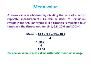
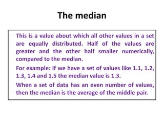
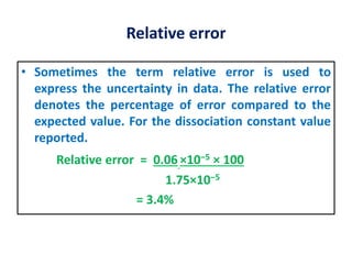
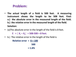
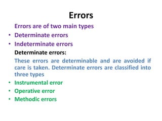
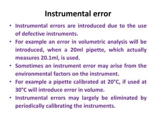
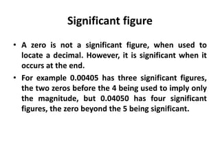
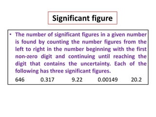
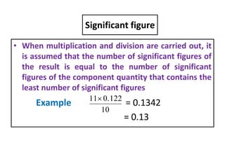
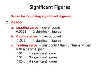
The document provides a comprehensive overview of concepts in analytical chemistry, including mean, median, accuracy, precision, and types of errors in chemical analysis. It distinguishes between determinate (instrumental, operative, methodic) and indeterminate errors while explaining how to calculate absolute and relative errors. Additionally, it addresses the importance of significant figures and the normal error curve in assessing measurement reliability.

1. ANALYTICAL CHEMISTRY
(Error in Chemical Analysis)
Dr.S.SURESH
Assistant Professor
Email:avitsureshindia@gmail.com

2. Mean value
A mean value is obtained by dividing the sum of a set of
replicate measurements by the number of individual
results in the set. For example, if a titration is repeated four
times and the titre values are 10.1, 9.9, 10.0 and 10.2ml
Mean = 10.1 + 9.9 + 10 + 10.2
4
= 40.2
4
= 10.05
This mean value is also called arithmetic mean or average.

3. The median
This is a value about which all other values in a set
are equally distributed. Half of the values are
greater and the other half smaller numerically,
compared to the median.
For example: If we have a set of values like 1.1, 1.2,
1.3, 1.4 and 1.5 the median value is 1.3.
When a set of data has an even number of values,
then the median is the average of the middle pair.

4. Accuracy
• Accuracy represents the nearness to a
measurement to its expected value. Any
difference between the measured value and
the expected value is expressed as error.
• For example: The dissociation constant for
acetic acid is 1.75×10‒5 at 25 °C. In an
experiment, if a student arrives at exactly this
value, his value is said to be accurate.

5. Precision
• Precision is defined as the agreement between the
numerical value of two or more measurements of
the same object that have been made in an
identical manner. Thus, a value is said to be precise,
when there is agreement between a set of results
for the same quantity.
• However a precise value need not be accurate.

6. Methods of expressing precision
• Precision can be expressed in an absolute method.
In the absolute way the deviation from the mean
│xi ‒ │ expresses precision without considering sign
_
X
S.No
Sample of an
organic compound
% of carbon
Deviation from mean
│xi ‒ │
1 X1 38.42 0.20
2 X2 38.02 0.20
3 X3 38.22 0.00
= 38.22
= 0.133
(Average deviation)
_
X
_
X
3
0.40

7. Absolute error
• The term accuracy is denoted in terms of
absolute error E, E is the difference between the
observed value (Xi) and the expected value (Xt).
E = │ Xi – Xt│
• If a student obtains a value of 1.69×10‒5 for the
dissociation constant of acetic acid at 25°C, the
absolute error in this determination is
E = │1.69×10‒5 – 1.75×10‒5 │
= │0.06 ×10‒5 │

8. Relative error
• Sometimes the term relative error is used to
express the uncertainty in data. The relative error
denotes the percentage of error compared to the
expected value. For the dissociation constant value
reported.
Relative error = 0.06 ×10‒5 × 100
1.75×10‒5
= 3.4%

9. Problem:
• The actual length of a field is 500 feet. A measuring
instrument shows the length to be 508 feet. Find:
a.) the absolute error in the measured length of the field.
b.) the relative error in the measured length of the field.
Solution:
• (a)The absolute error in the length of the field is 8 feet.
E = │ Xi – Xt│ = 508-500 = 8 feet.
• b.) The relative error in the length of the field is
Relative error = 8 × 100
500
= 1.6%

10. Errors
Errors are of two main types
• Determinate errors
• Indeterminate errors
Determinate errors:
These errors are determinable and are avoided if
care is taken. Determinate errors are classified into
three types
• Instrumental error
• Operative error
• Methodic errors

11. Instrumental error
• Instrumental errors are introduced due to the use
of defective instruments.
• For example an error in volumetric analysis will be
introduced, when a 20ml pipette, which actually
measures 20.1ml, is used.
• Sometimes an instrument error may arise from the
environmental factors on the instrument.
• For example a pipette calibrated at 20°C, if used at
30°C will introduce error in volume.
• Instrumental errors may largely be eliminated by
periodically calibrating the instruments.

12. Operative errors
• These errors are also called personal errors and are
introduced because of variation of personal
judgements.
• For example due to colour blindness a person may
arrive at wrong results in a volumetric or
colorimetric analysis.
• Using incorrect mathematical equations and
committing arithmetic mistakes will also cause
operative errors.

13. Methodic errors
• These errors are caused by adopting defective
experimental methods.
• For example in volumetric analysis the use of an
improper indicator leading to wrong results is an
example for methodic error.
• Proper understanding of the theoretical background
of the experiments is a necessity for avoiding
methodic errors.

14. Indeterminate errors
• These errors are also called accidental errors.
Indeterminate errors arise from uncertainties in
a measurement that are unknown and which
cannot be controlled by the experimentalist.
• For example: When pipetting out a liquid, the
speed of draining, the angle of holding the
pipette, the portion at which the pipette is held,
etc, would introduce indeterminate error in the
volume of the liquid pipette out.

15. Significant figure
• Data have to be reported with care keeping in mind
reliability about the number of figures used.
• For example, when reporting a value as many as six
decimal numbers can be obtained, when one uses a
calculator.
• However, reporting all these decimal numbers is
meaningless because, as is generally true, there may
be uncertainty about the first decimal itself.
• Therefore, experimental data should be rounded off.

16. Significant figure
• A zero is not a significant figure, when used to
locate a decimal. However, it is significant when it
occurs at the end.
• For example 0.00405 has three significant figures,
the two zeros before the 4 being used to imply only
the magnitude, but 0.04050 has four significant
figures, the zero beyond the 5 being significant.

17. Significant figure
• The number of significant figures in a given number
is found by counting the number figures from the
left to right in the number beginning with the first
non-zero digit and continuing until reaching the
digit that contains the uncertainty. Each of the
following has three significant figures.
646 0.317 9.22 0.00149 20.2

18. Significant figure
• When multiplication and division are carried out, it
is assumed that the number of significant figures of
the result is equal to the number of significant
figures of the component quantity that contains the
least number of significant figures
Example = 0.1342
= 0.13
10
0.12211

19. Significant Figures
Rules for Counting Significant Figures
2. Zeros
a. Leading zeros - never count
0.0025 2 significant figures
b. Captive zeros - always count
1.008 4 significant figures
c. Trailing zeros - count only if the number is written
with a decimal point
100 1 significant figure
100. 3 significant figures
120.0 4 significant figures

20. Normal error Curve
• The normal error curve was first studied by
Carl Friedrich Gauss as a curve for the
distribution of errors. He found that the
distribution of errors could be closely
approximated by a curve called the normal
curve of errors.

21. Normal error Curve
• This normal distribution curve is a useful one to
measure the extent of indeterminate error. It is
given by
is the standard deviation
x = value of the continuous random variable.
µ = mean of the normal random variable
π = constant = 3.14


22. Normal error Curve
• In normal error curve, the frequency is plotted
against mean deviation.
• When the frequency is maximum the error is nil.
• When the frequency decreases, the magnitude of
the error increases

23. Normal error Curve
• When is very large, the curve obtained is
bell shaped. When is very small, then a
sharp curve is obtained.
• When frequency increases, the will
decrease → sharp curve → nil error.
• When frequency decreases the will
increase → bell shaped curve → error
increases





24. Normal error Curve
• The normal distributions are extremely
important in statistics and are often used in
science for real valued random variables
whose distributions are not known.

25. • How many significant figures are in:
1. 12.548
2. 0.00335
3. 504.70
4. 4000
5. 0.10200

26. (1) There are 5. All numbers are significant.
(2) There are 3. The zeros before the number
is not significant.
(3) There are 5 significant figures.
(4) There is 1 significant figure.
(5) There are 5 significant figures.