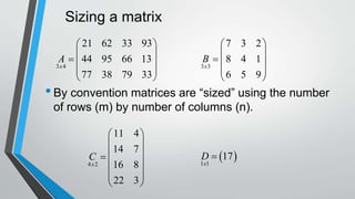
This document provides an introduction to matrices. It defines a matrix as a rectangular array of numbers or other items arranged in rows and columns. Matrices are conventionally sized using the number of rows and columns. The document outlines basic matrix operations such as addition, subtraction, scalar multiplication, and matrix multiplication. It also defines key matrix types including identity, diagonal, triangular, and transpose matrices.

1. 2018
Lecture №2
MATRICES
Dobroshtan Оlena

2. What is a matrix?
•A Matrix is just rectangular arrays of items
•A typical matrix is a rectangular array of numbers
arranged in rows and columns.
3 4
21 62 33 93
44 95 66 13
77 38 79 33
x
A
 
 
  
 
 

3. Sizing a matrix
•By convention matrices are “sized” using the number
of rows (m) by number of columns (n).
3 4
21 62 33 93
44 95 66 13
77 38 79 33
x
A
 
 
  
 
 
3 3
7 3 2
8 4 1
6 5 9
x
B
 
 
  
 
 
4 2
11 4
14 7
16 8
22 3
x
C
 
 
 
 
 
 
 1 1
17
x
D 

4. Two matrices A = [aij] and B = [bij] are said to be
(A = B) iff each element of A is equal to the
corresponding element of B, i.e., aij = bij for 1  i 
m, 1  j  n.
if A = B, it implies aij = bij for 1  i  m, 1  j  n;
if aij = bij for 1  i  m, 1  j  n, it implies A = B.

5. Given that A = B, find and .
1 0
4 2
A
 
  
 
a b
B
c d
 
  
 
if A = B, then and

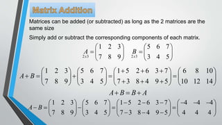
6. If A = [aij] and B = [bij] are m  n matrices, then
A + B is defined as a matrix C = A + B, where
C= [cij], cij = aij + bij for 1  i  m, 1  j  n.
Example: if and
Evaluate A + B and A – B.
1 2 3
0 1 4
A
 
  
 
2 3 0
1 2 5
B
 
  
 
1 2 2 3 3 0
0 ( 1) 1 2 4 5
A B
   
   
    
1 2 2 3 3 0
0 ( 1) 1 2 4 5
A B
   
   
    
3 5 3
1 3 9
 
 
 
1 1 3
1 1 1
  
 
  

7. Two matrices of the order are said to be
conformable for addition or subtraction.
Two matrices of orders cannot be added
or subtracted, e.g.,
2 3 7
1 1 5
 
 
 
1 3 1
2 1 4
4 7 6
 
 
 
 
 
are NOT conformable for addition or subtraction.

8. Matrices can be added (or subtracted) as long as the 2 matrices are the
same size
Simply add or subtract the corresponding components of each matrix.
2 3 2 3
1 2 3 5 6 7
7 8 9 3 4 5x x
A B
   
    
   
1 2 3 5 6 7 1 5 2 6 3 7 6 8 10
7 8 9 3 4 5 7 3 8 4 9 5 10 12 14
A B
         
           
         
A B B A  
1 2 3 5 6 7 1 5 2 6 3 7 4 4 4
7 8 9 3 4 5 7 3 8 4 9 5 4 4 4
A B
            
           
         

9. Let l be any scalar and A = [aij] is an m  n matrix.
Then lA = [laij] for 1  i  m, 1  j  n, i.e., each
element in A is multiplied by l.
1 2 3
0 1 4
A
 
  
 
Example: . Evaluate 3A.
3 1 3 2 3 3
3
3 0 3 1 3 4
A
   
  
   
In particular, l = -1, i.e., -A = [-aij]. It’s called the
. Note: A - A = 0 is a zero matrix
3 6 9
0 3 12
 
 
 

10. Matrices A, B and C are conformable,
A + B = B + A
A + (B +C) = (A + B) +C
l(A + B) = lA + lB, where l is a scalar
(commutative law)
(associative law)
(distributive law)

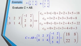
11. If A = [aij] is a m  p matrix and B = [bij] is a p  n
matrix, then AB is defined as a m  n matrix C = AB,
where C= [cij] with
1 1 2 2
1
...

    
p
ij ik kj i j i j ip pj
k
c a b a b a b a b
1 2 3
0 1 4
A
 
  
 
1 2
2 3
5 0
B
 
 
  
 
 
, and C = AB.
Evaluate c21.
1 2
1 2 3
2 3
0 1 4
5 0
 
  
  
  
 
21 0 ( 1) 1 2 4 5 22       c
for 1  i  m, 1  j  n.

12. 1 2 3
0 1 4
A
 
  
 
1 2
2 3
5 0
B
 
 
  
 
 
11
12
21
22
1 ( 1) 2 2 3 5 18
1 2
1 2 2 3 3 0 81 2 3
2 3
0 ( 1) 1 2 4 5 220 1 4
5 0
0 2 1 3 4 0 3
c
c
c
c
       
            
              
         
1 2
1 2 3
2 3
0 1 4
5 0
C AB
 
  
    
  
 
18 8
22 3
 
 
 
Evaluate C = AB.

13. Properties
Matrices A, B and C are conformable,
A(B + C) = AB + AC
(A + B)C = AC + BC
A(BC) = (AB) C
AB  BA in general
AB = 0 NOT necessarily imply A = 0 or B = 0
AB = AC NOT necessarily imply B = C

14. 1
4
A square matrix whose elements aij = 0,
for i > j is called upper triangular, i.e.,
11 12 1
22 20
0 0
n
n
nn
a a a
a a
a
 
 
 
 
 
 
A square matrix whose elements aij = 0,
for i < j is called lower triangular, i.e.,
11
21 22
1 2
0 0
0
n n nn
a
a a
a a a
 
 
 
 
 
 

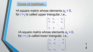
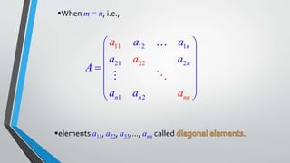
15. Both upper and lower triangular, i.e., aij = 0, for i  j , i.e.,
11
22
0 0
0 0
0 0 nn
a
a
D
a
 
 
 
 
 
 
11 22diag[ , ,..., ] nnD a a a
is called a , simply

16. When m = n, i.e.,
elements a11, a22, a33,…, ann called .
12 1
21 2
1 2
11
22
n
n
n n nn
a a a
a a
A
a a
a
a
 
 
 
 
 
 

17. In particular, a11 = a22 = … = ann = 1, the matrix is called
.
Properties: AE= EA = A
of identity matrices:
1 0
0 1
 
 
 
1 0 0
0 1 0
0 0 1
 
 
 
  

18. Matrix Transpose: is the mxn matrix obtained by
interchanging the rows and columns of a matrix (converting
it to an nxm matrix)
 4 1 1 4
12
9
12 9 4 0
4
0
T
x x
X X
 
 
   
 
 
 
3 4 4 3
21 44 77
21 62 33 93
62 95 38
44 95 66 13 '
33 66 79
77 38 79 33
93 13 33
x x
A A
 
   
           
 

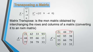
19. The matrix obtained by interchanging the rows and
columns of a matrix A is called the transpose of A
(write AT).
Example:
The transpose of A is
1 2 3
4 5 6
 
  
 
A
1 4
2 5
3 6
 
   
  
T
A
For a matrix A = [aij], its transpose AT = [bij], where
bij = aji.

20. A matrix A such that AT = A is called symmetric,
i.e., aji = aij for all i and j.
A + AT must be .
1 2 3
2 4 5
3 5 6
A
 
 
  
  

21. A matrix A is called orthogonal if AAT = ATA = I, i.e.,
AT = A-1
prove that is orthogonal.
1/ 3 1/ 6 1/ 2
1/ 3 2 / 6 0
1/ 3 1/ 6 1/ 2
A
 
 
  
 
 
 
Since, . Hence, AAT = ATA = E.
1/ 3 1/ 3 1/ 3
1/ 6 2/ 6 1/ 6
1/ 2 0 1/ 2
T
A
 
 
  
 
  

22. (AB)-1 = B-1A-1
(AT)T = A and (lA)T = l AT
(A + B)T = AT + BT
(AB)T = BT AT

23. Cofactor matrix of
1 2 3
0 4 5
1 0 6
A
 
 
  
 
 
The cofactor for each element of matrix A:
11
4 5
24
0 6
A   12
0 5
5
1 6
A    13
0 4
4
1 0
A   
21
2 3
12
0 6
A   
22
1 3
3
1 6
A   23
1 2
2
1 0
A   
31
2 3
2
4 5
A   
32
1 3
5
0 5
A    
33
1 2
4
0 4
A  

24. Cofactor matrix of is then given by:
1 2 3
0 4 5
1 0 6
A
 
 
  
 
 
24 5 4
12 3 2
2 5 4


 
 
 
 
 
 

25. Inverse matrix of is given by:
1 2 3
0 4 5
1 0 6
A
 
   
  
1
24 5 4 24 12 2
1 1
12 3 2 5 3 5
22
2 5 4 4 2 4
T
A
A

     
         
        
12 11 6 11 1 11
5 22 3 22 5 22
2 11 1 11 2 11
  
   
  