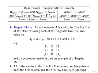
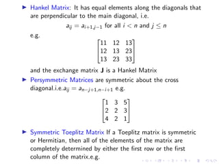
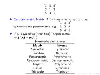
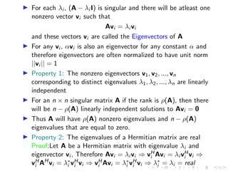
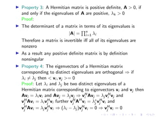
The document provides an in-depth overview of linear algebra concepts relevant to signal engineering and machine learning, covering topics such as vectors, norms, inner products, matrices, and linear equations. It explains definitions and properties, including linear independence, matrix inversion, determinants, and the formulation of linear equations in matrix form. Various special matrix forms, their properties, and applications in FIR filters are also discussed.

1. Linear Algebra for Signal Engineers, AI & ML
Enthusiasts
By
Sandip Kumar Ladi

2. Vectors
▶ A vector is an array of real valued or complex valued numbers
or functions
▶ Vectors usually represented by lowercase bold letters, e.g. x, a
and v
▶ such vectors are assumed to be column vectors, e.g.
x =






x1
x2
:
:
xN






is a column vector containing N real or complex scalars
corresponding to real or complex vector
▶ The transpose of a vector xT is a row vector
xT
=
x1 x2 .... xN

3. ▶ The Hermitian transpose xH is the complex conjugate of the
transpose of x
xH
= (xT
)∗
=
x∗
1 x∗
2 .... x∗
N
▶ As an example a finite duration sequence of length N may be
represented in vector form as
x =






x(0)
x(1)
:
:
x(N − 1)






The distance metric or norm
1. The Euclidean or L2 norm of a vector x of dimension N is
||x||2 =
v
u
u
t
N
X
i=1
|xi |2

4. 2. The L1 norm
||x||1 =
N
X
i=1
|xi |
3. The L∞ norm
||x||∞ = max
i
|xi |
▶ Assuming ||x|| ̸= 0 the normalized vector or the unit norm
vector is
vx =
x
||x||
and it lies in the same direction as x
▶ if the elements of a vector x are signal values of a discrete
time signal x(n) then the square of the L2 norm of x
||x||2
=
N−1
X
n=0
|x(n)|2
is energy of the signal
▶ norm as measure of distance between two vectors
d(x, y) = ||x − y|| =
qPN
i=1 |xi − yi |2

5. Inner Product
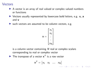
▶ If a = [a1, ...., aN]T and b = [b1, ...., bN]T are two complex
vectors, the Inner Product is a scalar defined by
a, b = aH
b =
N
X
i=1
a∗
i bi
for real vectors inner product simplifies to
a, b = aT
b =
N
X
i=1
ai bi
▶ Inner product defines the geometrical relationship between
two vectors, which is given by
a, b = ||a|| ||b|| cos θ
θ: angle between the two vectors
▶ Orthogonal vectors: a ̸= 0 and b ̸= 0 but a, b = 0
▶ Orthonormal vectors: a, b = 0 and ||a|| = 1, ||b|| = 1

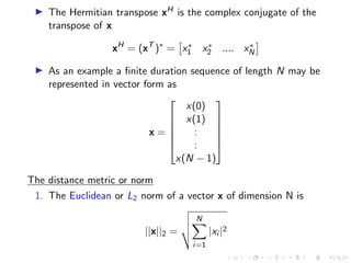
6. ▶ The inner product between two vectors is bounded by the
product of their magnitudes
| a, b | ≤ ||a|| ||b||
equality holds when both the vectors are colinear (a = αb for
some constant α) and the above inequality is referred to as
Cauchy-Scwartz inequality
▶ Since ||a ± b||2 = ||a||2 ± 2 a, b +||b||2 ≥ 0 it follows
that
2| a, b | ≤ ||a||2
+ ||b||2
▶ Writing the sample response of an FIR filter h(n) in vector
form given below
h = [h(0), h(1), ..., h(N − 1)]T
The output y(n) of the FIR filter may be written as the inner
product
y(n) =
N−1
X
k=0
h(k)x(n − k) = hT
x(n)
where x(n) = [x(n), x(n − 1), ..., x(n − N + 1)]T

7. Linear Independence
▶ A set of n vectors v1,v2,...,vn is said to be linearly
independent if
α1v1 + α2v2 + ... + αnvn = 0
implies that αi = 0 for all i
▶ If a set of nonzero αi can be found so that above equation
holds then the set is said to be linearly dependent
▶ If v1,v2,...,vn is a set of linearly dependent vectors, then
atleast one of the vectors may be expressed as a linear
combination of the remaining vectors e.g.
v1 = β2v2 + β3v3 + ... + βnvn
for some set of scalars βi
▶ For vectors of dimension N, no more than N vectors may be
linearly independent which implies any set containing more
than N vectors will always be linearly dependent

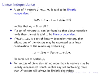
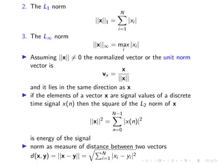
8. Vector Spaces and Basis Vectors
▶ Given a set of N vectors V = {v1, v2, ..., vN}, consider the set
of all vectors V that may be formed from a linear combination
of vectors vi i.e. v =
PN
i=1 αi vi and v ∈ V
▶ This set V forms a vector space
▶ The vectors vi are said to span the space V
▶ If the vectors vi are linearly independent then they are said to
form a basis for the space V
▶ The number of vectors in the basis, N, is referred to as the
dimension of the vector space V
▶ Example The set of all real vectors of the form
x = [x1, x2, ..., xN]T forms an N-dimensional vector
space,denoted by RN, that is spanned by the basis vectors,
u1 = [1, 0, 0, ..., 0]T ,u2 = [0, 1, 0, ..., 0]T ,...,uN =
[0, 0, 0, ..., 1]T . In terms of this basis, any vector
v = [v1, v2, ..., vn]T ∈ RN may be uniquely decomposed as
v =
PN
i=1 vi ui
Note:The basis for a vector space is not unique.

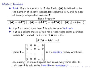
9. Matrices
▶ An n × m matrix is an array of numbers(real or complex)
functions having n rows and m columns.e.g.
A = [aij ] =






a11 a12 .. a1m
a21 a22 .. a2m
. . .
. . .
an1 an2 .. anm






is an n × m matrix of numbers aij and
A(z) = [aij (z)] =






a11(z) a12(z) .. a1m(z)
a21(z) a22(z) .. a2m(z)
. . .
. . .
an1(z) an2(z) .. anm(z)






is an n × m matrix of functions aij (z)
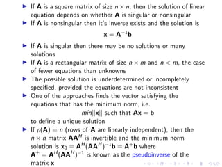
▶ If n = m then A is a n × n square matrix of n rows and n
columns

10. ▶ Example: The output of an FIR-LTI filter with a unit sample
response h(n) may be written in vector form as
y(n) = hT
x(n) = xT
(n)h
if x(n) = 0 for n 0, then we may express y(n) for n ≥ 0 as
X0h = y, where X0 is a convolution matrix defined by
X0 =












x(0) 0 0 .. 0
x(1) x(0) 0 .. 0
x(2) x(1) x(0) .. 0
. . . .
. . . .
x(N − 1) x(N − 2) x(N − 3) .. x(0)
. . . .
. . . .












and y = [y(0), y(1), y(2), ...]T
Note: The elements of X0 in each diagonal are same. X0 has
N − 1 columns and an infinite number of rows.

11. ▶ Matrices can also be represented as a set of column vectors or
row vectors, such as A = [c1, c2, ..., cm] or A =






rH
1
rH
2
.
.
rH
n






▶ A matrix may also be partitioned into submatrices. For
instance the matrix A may be partitioned into
A =
A11 A12
A21 A22
where A11 is p × q,A12 is p × (m − q),A21
is (n − p) × q and A22 is (n − p) × (m − q)
▶ If A is an n × m matrix, then the transpose denoted by AT
is
the m × n matrix that is formed by interchanging the rows
and columns of A
▶ Symmetric matrix: For a square matrix if A = AT
▶ Hermitian Transpose:AH
= (A∗
)T
= (AT
)
∗
▶ Hermitian matrix: For a square complex valued matrix if
A = AH
▶ Properties: (A + B)H = AH
+ BH
, (AH
)H = A and
(AB)H = BH
AH

12. Matrix Inverse
▶ Rank: For a n × m matrix A the Rank ρ(A) is defined to be
the number of linearly independent columns in A and number
of linearly independent rows in A
Rank Property
ρ(A) = ρ(AH
) ρ(A) = ρ(AAH
) = ρ(AH
A) ρ(A) ≤ min(m, n)
▶ If ρ(A) = min(m, n) then A is said to be of full rank
▶ If A is a square matrix of full rank, then there exists a unique
matrix A−1
, called the inverse of A such that
A−1
A = AA−1
= I
where I =






1 0 0 .. 0
0 1 0 .. 0
. . . .
. . . .
0 0 0 .. 1






is the identity matrix which has
ones along the main diagonal and zeros everywhere else. In
this case A is said to be invertible or nonsingular

13. ▶ If A is not of full rank (ρ(A) n) then it is said to be
noninvertible or singular and A does not have an inverse
Matrix Inverse Property (A and B are invertible)
(AB)−1 = B−1
A−1
(AH
)−1 = (A−1
)H
▶ Matrix Inversion Lemma:
(A + BCD)−1
= A−1
− A−1
B(C−1
+ DA−1
B)DA−1
▶ The Determinant: If A = a11 is a 1 × 1 matrix, then it’s
determinant is defined to be det(A) = a11. The determinant
of an n × n matrix is defined recursively in terms of the
determinants of (n − 1) × (n − 1) matrices as below. For any j
det(A) =
n
X
i=1
(−1)i+j
aij det(Aij )
where Aij is the (n − 1) × (n − 1) matrix that is formed by
deleting the ith row and the jth column of A
▶ Trace Given an n × n matrix A, the trace is the sum of the
terms along the diagonal i.e. tr(A) =
Pn
i=1 aii
Note: An n × n matrix is invertible if and only if det(A) ̸= 0

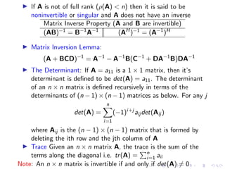
14. Determinant Property
det(AB) = det(A)det(B) det(αA) = αndet(A)
det(A−1
) = 1
det(A),A is invertible det(AT
) = det(A)
▶ Example For a 2 × 2 matrix
A =
a11 a12
a21 a22
det(A) = a11a22 − a12a21
and for a 3 × 3 matrix
A =


a11 a12 a13
a21 a22 a23
a31 a32 a33


det(A) = a11det
a22 a23
a32 a33
−a12det
a21 a23
a31 a33
+a13det
a21 a22
a31 a32
= a11[a22a33−a23a32]−a12[a21a33−a31a23]+a13[a21a32−a31a22]

15. Linear Equations
▶ Consider the following set of n linear equations in the m
unknowns xi , i = 1, 2, ..., m
a11x1 + a12x2 + ... + a1mxm = b1
a21x1 + a22x2 + ... + a2mxm = b2
.
.
.
an1x1 + an2x2 + ... + anmxm = bn
These equations may be written in matrix form as
Ax = b
A is an m × n matrix with entries aij , x is an m-dimensional
vector containing the unknown xi and b is an n-dimensional
vector with elements bj
▶ An alternative representation in terms of column vectors ai of
the matrix A is
b =
m
X
i=1
xi ai

16. ▶ If A is a square matrix of size n × n, then the solution of linear
equation depends on whether A is singular or nonsingular
▶ If A is nonsingular then it’s inverse exists and the solution is
x = A−1
b
▶ If A is singular then there may be no solutions or many
solutions
▶ If A is a rectangular matrix of size n × m and n m, the case
of fewer equations than unknowns
▶ The possible solution is underdetermined or incompletely
specified, provided the equations are not inconsistent
▶ One of the approaches finds the vector satisfying the
equations that has the minimum norm, i.e.
min||x|| such that Ax = b
to define a unique solution
▶ If ρ(A) = n (rows of A are linearly independent), then the
n × n matrix AAH
is invertible and the minimum norm
solution is x0 = AH
(AAH
)−1b = A+
b where
A+
= AH
(AAH
)−1 is known as the pseudoinverse of the
matrix x

17. ▶ If m n then there are more equations than unknowns for
which in general no solution exists. Here the equations are
inconsistent and the solution is said to be overdetermined
▶ Here the arbitrary vector b cannot be represented in terms of
a linear combination of the columns of A. Hence the goal is
to find the coefficient xi that produces the best approximation
b̂ to b, i.e.
b̂ =
m
X
i=1
xi ai
▶ A common approach is to find the least squares solution, i.e.
the vector x that minimizes the norm of the error
||e||2 = ||b − Ax||2
▶ Least square solution has the property that the error
e = b − Ax is orthogonal to each of the Vectors that are used
in the approximation for b,i.e. the column vectors of A.This
orthogonality implies
AH
e = 0 ⇒ AH
Ax = AH
b
▶ If A is full rank, AH
A is invertible, x0 = (AH
A)−1AH
b = A+
b

18. ▶ The best approximation b̂ to b is given by the projection of
the vector b onto the subspace spanned by the vector ai
b̂ = Ax0 = A(AH
A)−1
AH
b = AA+
b = PAb
where PA = AA+
is called the projection matrix
▶ Finally the minimum least square error is
min||e||2
= bH
e = bH
b − bH
Ax0
Special Matrix Forms
▶ Diagonal Matrix is a square matrix which has all of its entries
equal to zero except possibly those along the main diagonal.
It is of the form
A = diag{a11, a22, ..., ann} =





a11 0 ... 0
0 a22 ... 0
.
.
.
.
.
.
.
.
.
0 0 ... ann





▶ As a special case Identity Matrix I = diag{1, 1, ..., 1}
▶ block diagonal matrix: If A = diag{A11, A22, ..., Akk}, where
the entries along the diagonal Akk’s are matrices

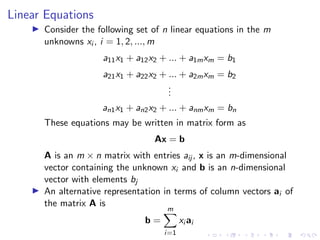
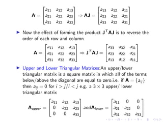
19. ▶ Exchange Matrix: It is symmetric and has ones along the
cross diagonal and zeros everywhere else.i.e.
J =





0 ... 0 1
0 ... 1 0
.
.
.
.
.
.
.
.
.
1 ... 0 0





▶ Interestingly J2
= I and J−1
= J
▶ when we post multiply a vector v by the exchange matrix J
the order of the entries of v will reverse. i.e.
J[v1, v2, ..., vn]T
= [vn, vn−1, ..., v1]
▶ If a matrix A is multiplied on the left by the exchange matrix,
the operation would reverse the order of each column. e.g.
A =


a11 a12 a13
a21 a22 a23
a31 a32 a33

 ⇒ JT
A =


a31 a32 a33
a21 a22 a23
a11 a12 a13


▶ Similarly if A is multiplied on the right by J, then the order of
the entries in each row is reversed

20. A =


a11 a12 a13
a21 a22 a23
a31 a32 a33

 ⇒ AJ =


a13 a12 a11
a23 a22 a21
a33 a32 a31


▶ Now the effect of forming the product JT
AJ is to reverse the
order of each row and column
A =


a11 a12 a13
a21 a22 a23
a31 a32 a33

 ⇒ JT
AJ =


a33 a32 a31
a23 a22 a21
a13 a12 a11


▶ Upper and Lower Triangular Matrices:An upper/lower
triangular matrix is a square matrix in which all of the terms
below/above the diagonal are equal to zero.i.e. if A = {aij }
then aij = 0 for i j/i j e.g. a 3 × 3 upper/ lower
triangular matrix
Aupper =


a11 a12 a13
0 a22 a23
0 0 a33

 andAlower =


a11 0 0
a21 a22 0
a31 a32 a33



21. Upper/Lower Triangular Matrix Property
AT
lower = Aupper and AT
upper = Alower upper−1 = upper
det(Alower ) or det(Aupper ) =
Qn
i=1 aii upper × upper = upper
lower × lower = lower lower−1 = lower
▶ Toeplitz Matrix: An n × n matrix A is said to be Toeplitz if all
of the elements along each of the diagonals have the same
value i.e.
aij = ai+1,j+1 for all i n and j n
e.g. 

11 12 13
21 11 12
31 21 11


and a convolution matrix is also an example of a Toeplitz
Matrix
▶ All of the entries in the Toeplitz Matrix are completely defined
once the first column and the first row have been specified

22. ▶ Hankel Matrix: It has equal elements along the diagonals that
are perpendicular to the main diagonal, i.e.
aij = ai+1,j−1 for all i n and j ≤ n
e.g. 

11 12 13
12 13 23
13 23 33


and the exchange matrix J is a Hankel Matrix
▶ Persymmetric Matrices are symmetric about the cross
diagonal.i.e.aij = an−j+1,n−i+1 e.g.


1 3 5
2 2 3
4 2 1


▶ Symmetric Toeplitz Matrix If a Toeplitz matrix is symmetric
or Hermitian, then all of the elements of the matrix are
completely determined by either the first row or the first
column of the matrix.e.g.

23. 

1 3 5
3 1 3
5 3 1


▶ Centrosymmetric Matrix: A Centrosymmetric matrix is both
symmetric and persymmetric. e.g.


1 3 5
3 2 4
5 4 1


▶ If A is symmetric(Hermitian) Toeplitz matrix
⇒ JT
AJ = A(A∗
)
Symmetries and Inverses
Matrix Inverse
Symmetric Symmetric
Hermitian Hermitian
Persymmetric Persymmetric
Centrosymmetric Centrosymmetric
Toeplitz Persymmetric
Hankel Symmetric
Triangular Triangular

24. ▶ Orthogonal Matrix: A real n × n matrix is said to be
orthogonal if the columns(and rows) are orthonormal. i.e. if
the columns of A are ai then
A = [a1, a2, ..., an] and aT
i ai =
(
1 i = j
0 i ̸= j
▶ If A is orthogonal then AT
A = I, thus the inverse A−1
= AT
▶ Example:Exchange Matrix J is an orthogonal Matrix since
JT
J = J2
= I
▶ In a complex n × n Matrix A, if the columns(rows) are
orthogonal
aH
i ai =
(
1 i = j
0 i ̸= j
which implies AH
A = I and A is said to be Unitary matrix
▶ The inverse of a unitary matrix is same as its Hermitian
transpose
A−1
= AH

25. Quadratic and Hermitian Forms
▶ The quadratic form of a n × n real symmetric matrix A and a
n × n Hermitian matrix C is a scalar and is respectively
defined by
QA(x) = xT Ax =
Pn
i=1
Pn
j=1 xi aij xj
and
QC (x) = xHCx =
Pn
i=1
Pn
j=1 x∗
i aij xj
where xT = [x1, x2, ..., xn] is a vector of n real variables and
also the quadratic form is a quadratic function in the n
variables x1, x2, ..., xn
▶ Example: The quadratic form of A =
2 −1
1 2
is
QA(x) = xT Ax = 2x2
1 + 2x2
2
▶ For any x ̸= 0
Definiteness condition Definiteness condition
+ve definite QA(x) 0 -ve Semidefinite QA(x) ≤ 0
+ve semidefinite QA(x) ≥ 0 indefinite none of above
-ve definite QA(x) 0

26. Eigenvalues and Eigenvectors
▶ Preliminary: For any n × n matrix A and for any n × m full
rank matrix B, the definiteness of A and BH
AB will be the
same
Proof:If A 0 and B is full rank, then BH
AB 0 since for
any vector x,
xH(BH
AB)x = (Bx)HA(Bx) = vHAv
where v = Bx. Hence, if A 0, then vHAv 0 and
BH
AB 0 is positive definite (v = Bx is nonzero for any
nonzero vector x)
▶ Let A be an n × n matrix and considering the following set of
linear equations
Av = λv ⇒ (A − λI)v = 0
for a nonzero vector v to be a solution A − λI need to be
singular, in other words
p(λ) = |A − λI| = 0
p(λ) is the n-th order Characteristic polynomial of the matrix
A and the roots λi , i = 1, 2, ..., n are called the Eigenvalues of
A

27. ▶ For each λi , (A − λi I) is singular and there will be atleast one
nonzero vector vi such that
Avi = λi vi
and these vectors vi are called the Eigenvectors of A
▶ For any vi , αvi is also an eigenvector for any constant α and
therefore eigenvectors are often normalized to have unit norm
||vi || = 1
▶ Property 1: The nonzero eigenvectors v1, v2, ..., vn
corresponding to distinct eigenvalues λ1, λ2, ..., λn are linearly
independent
▶ For an n × n singular matrix A if the rank is ρ(A), then there
will be n − ρ(A) linearly independent solutions to Avi = 0
▶ Thus A will have ρ(A) nonzero eigenvalues and n − ρ(A)
eigenvalues that are equal to zero.
▶ Property 2: The eigenvalues of a Hermitian matrix are real
Proof:Let A be a Hermitian matrix with eigenvalue λi and
eigenvector vi , Therefore Avi = λi vi ⇒ vH
i Avi = λi vH
i vi ⇒
vH
i AH
vi = λ∗
i vH
i vi ⇒ vH
i Avi = λ∗
i vH
i vi ⇒ λ∗
i = λi = real

28. ▶ Property 3: A Hermitian matrix is positive definite, A 0, if
and only if the eigenvalues of A are positive, λk 0
Proof:
▶ The determinant of a matrix in terms of its eigenvalues is
|A| =
Qn
i=1 λi
Therefore a matrix is invertible iff all of its eigenvalues are
nonzero
▶ As a result any positive definite matrix is by definition
nonsingular
▶ Property 4: The eigenvectors of a Hermitian matrix
corresponding to distinct eigenvalues are orthogonal ⇒ if
λi ̸= λj then vi , vj = 0
Proof: Let λi and λj be two distinct eigenvalues of a
Hermitian matrix corresponding to eigenvectors vi and vj then
Avi = λi vi and Avj = λj vj ⇒ vH
i Avj = λj vH
i vj and
vH
j Avi = λi vH
j vi further vH
j AH
vi = λ∗
j vH
j vi and
vH
j Avi = λj vH
j vi ⇒ (λi − λj )vH
j vi = 0 ⇒ vH
j vi = 0

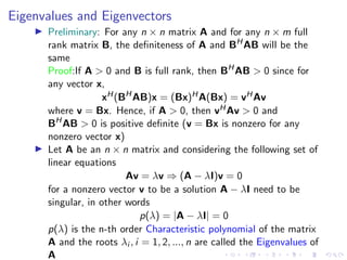
29. Eigenvalue Decomposition
▶ Let A be an n × n matrix with eigenvalues λk and
eigenvectors vk then
Avk = λkvk for k = 1, 2, ..., n
Matrix form of these n equations are as under
A[v1, v2, ...vn] = [λ1v1, λ2v2, ...λnvn]
Substituting V = [v1, v2, ..., vn] and Λ = diag{λ1, λ2, ..., λn}
we get
AV = VΛ
If the eigenvectors vi are independent then V is invertible and
the decomposition is as follows
A = VΛV−1
▶ Spectral Theorem When a matrix A is Hermitian then V is
unitary and the Eigenvalue Decomposition becomes
A = VΛVH
=
Pn
i=1 λi vi vH
i
This simplified Eigenvalue Decomposition is known as
Spectral Theorem where λi being the eigenvalues and vi are a
set of orthonormal vectors of A

30. ▶ For a nonsingular Hermitian Matrix A The inverse can be
obtained by using the spectral Theorem as follows
A−1
= (VΛVH
)−1 = (VH
)−1Λ−1V−1
= VΛ−1VH
=
Pn
i=1
1
λi
vi vH
i
This sum is always well defined since A is invertible
▶ Property 5:Let B be an n × n matrix with eigenvalues λi and
let A = B + αI then A and B have the same eigenvectors and
the eigenvalues of A are λi + α
Proof:Avk = (B + αI)vk = Bvk + αvk = (λk + α)vk