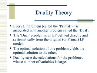
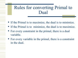
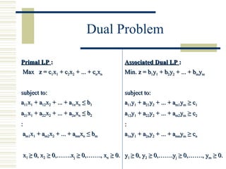
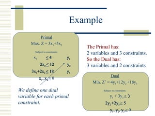
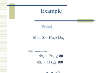
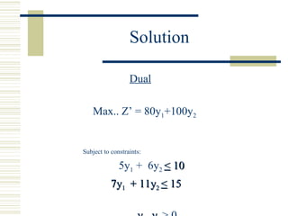
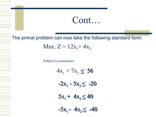
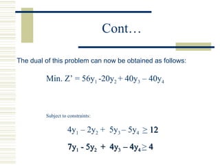
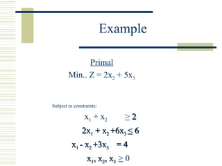
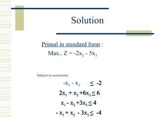
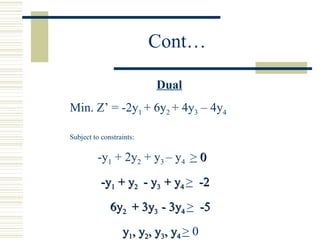
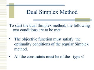
- Duality theory states that every linear programming (LP) problem has a corresponding dual problem, and the optimal solutions of the primal and dual problems are related. - The dual problem is obtained by converting the constraints of the primal to variables and vice versa. - The dual simplex method starts with an infeasible but optimal solution and moves toward feasibility while maintaining optimality, unlike the regular simplex method which moves from a feasible to optimal solution.

1. DUALITY

2. Duality Theory Every LP problem (called the ‘Primal’) has associated with another problem called the ‘Dual’. The ‘Dual’ problem is an LP defined directly and systematically from the original (or Primal) LP model. The optimal solution of one problem yields the optimal solution to the other. Duality ease the calculations for the problems, whose number of variables is large.

3. Rules for converting Primal to Dual If the Primal is to maximize, the dual is to minimize. If the Primal is to minimize, the dual is to maximize. For every constraint in the primal, there is a dual variable. For every variable in the primal, there is a constraint in the dual.

4. Dual Problem Primal LP : Max z = c 1 x 1 + c 2 x 2 + ... + c n x n subject to: a 11 x 1 + a 12 x 2 + ... + a 1n x n ≤ b 1 a 21 x 1 + a 22 x 2 + ... + a 2n x n ≤ b 2 : a m1 x 1 + a m2 x 2 + ... + a mn x n ≤ b m x 1 ≥ 0, x 2 ≥ 0,…….x j ≥ 0,……., x n ≥ 0. Associated Dual LP : Min. z = b 1 y 1 + b 2 y 2 + ... + b m y m subject to: a 11 y 1 + a 21 y 2 + ... + a m1 y m ≥ c 1 a 12 y 1 + a 22 y 2 + ... + a m2 y m ≥ c 2 : a 1n y 1 + a 2n y 2 + ... + a mn y m ≥ c n y 1 ≥ 0, y 2 ≥ 0,…….y j ≥ 0,……., y m ≥ 0.

5. Example Primal Max. Z = 3x 1 +5x 2 Subject to constraints: x 1 < 4 y 1 2x 2 < 12 y 2 3x 1 +2x 2 < 18 y 3 x 1 , x 2 > 0 The Primal has: 2 variables and 3 constraints. So the Dual has: 3 variables and 2 constraints Dual Min. Z’ = 4y 1 +12y 2 +18y 3 Subject to constraints: y 1 + 3y 3 > 3 2y 2 +2y 3 > 5 y 1 , y 2 , y 3 > 0 We define one dual variable for each primal constraint.

6. Example Primal Min.. Z = 10x 1 +15x 2 Subject to constraints: 5x 1 + 7x 2 > 80 6x 1 + 11x 2 > 100 x 1 , x 2 > 0

7. Solution Dual Max.. Z’ = 80y 1 +100y 2 Subject to constraints: 5y 1 + 6y 2 < 10 7y 1 + 11y 2 < 15 y 1 , y 2 > 0

8. Example Primal Max. Z = 12x 1 + 4x 2 Subject to constraints: 4x 1 + 7x 2 < 56 2x 1 + 5x 2 > 20 5x 1 + 4x 2 = 40 x 1 , x 2 > 0

9. Solution The equality constraint 5x 1 + 4x 2 = 40 can be replaced by the following two inequality constraints: 5x 1 + 4x 2 < 40 5x 1 + 4x 2 > 40 -5x 1 - 4x 2 < -40 The second inequality 2x 1 + 5x 2 > 20 can be changed to the less-than-or-equal-to type by multiplying both sides of the inequality by -1 and reversing the direction of the inequality; that is, -2x 1 - 5x 2 < -20

10. Cont… The primal problem can now take the following standard form: Max. Z = 12x 1 + 4x 2 Subject to constraints: 4x 1 + 7x 2 < 56 -2x 1 - 5x 2 < -20 5x 1 + 4x 2 < 40 -5x 1 - 4x 2 < -40 x 1 , x 2 > 0

11. Cont… Min. Z’ = 56y 1 -20y 2 + 40y 3 – 40y 4 Subject to constraints: 4y 1 – 2y 2 + 5y 3 – 5y 4 > 12 7y 1 - 5y 2 + 4y 3 – 4y 4 > 4 y 1 , y 2 , y 3 , y 4 > 0 The dual of this problem can now be obtained as follows:

12. Example Primal Min.. Z = 2x 2 + 5x 3 Subject to constraints: x 1 + x 2 > 2 2x 1 + x 2 +6x 3 < 6 x 1 - x 2 +3x 3 = 4 x 1 , x 2 , x 3 > 0

13. Solution Primal in standard form : Max.. Z = -2x 2 - 5x 3 Subject to constraints: -x 1 - x 2 < -2 2x 1 + x 2 +6x 3 < 6 x 1 - x 2 +3x 3 < 4 - x 1 + x 2 - 3x 3 < -4 x 1 , x 2 , x 3 > 0

14. Cont… Dual Min. Z’ = -2y 1 + 6y 2 + 4y 3 – 4y 4 Subject to constraints: -y 1 + 2y 2 + y 3 – y 4 > 0 -y 1 + y 2 - y 3 + y 4 > -2 6y 2 + 3y 3 - 3y 4 > -5 y 1 , y 2 , y 3 , y 4 > 0

15. DUAL SIMPLEX METHOD

16. Introduction Suppose a “basic solution” satisfies the optimality condition but not feasible, then we apply dual simplex method. In regular Simplex method, we start with a Basic Feasible solution (which is not optimal) and move towards optimality always retaining feasibility. In the dual simplex method, the exact opposite occurs. We start with a “optimal” solution (which is not feasible) and move towards feasibility always retaining optimality condition.The algorithm ends once we obtain feasibility.

17. Dual Simplex Method To start the dual Simplex method, the following two conditions are to be met: The objective function must satisfy the optimality conditions of the regular Simplex method. All the constraints must be of the type  .

18. Example Min. Z = 3x 1 + 2x 2 Subject to constraints: 3x 1 + x 2 > 3 4x 1 + 3x 2 > 6 x 1 + x 2 < 3 x 1 , x 2 > 0

19. Cont… Step I: The first two inequalities are multiplied by –1 to convert them to < constraints and convert the objective function into maximization function. Max. Z’ = -3x 1 - 2x 2 where Z’= -Z Subject to constraints: -3x 1 - x 2 < -3 -4x 1 - 3x 2 < -6 x 1 + x 2 < 3 x 1 , x 2 > 0

20. Cont… Let S 1 , S 2 , S 3 be three slack variables Model can rewritten as: Z’ + 3x 1 + 2x 2 = 0 -3x 1 - x 2 +S 1 = -3 -4x 1 - 3x 2 +S 2 = -6 x 1 + x 2 +S 3 = 3 Initial BS is : x 1 = 0, x 2 = 0, S 1 = -3, S 2 = -6, S 3 = 3 and Z=0.

21. Cont… Initial Basic Solution is Optimal (as the optimality condition is satisfied) but infeasible. Choose the most negative basic variable. Therefore, S 2 is the departing variable. Calculate Ratio = |Z row / S 2 row| (S 2 < 0) Choose minimum ratio. Therefore, x 2 is the entering variable. - - - 2/3 3/4 - Ratio 3 1 0 0 1 1 0 S 3 -6 0 1 0 -3 -4 0 S 2 -3 0 0 1 -1 -3 0 S 1 0 0 0 0 2 3 1 Z Sol. S 3 S 2 S 1 x 2 x 1 Z Coefficients of: Basic Variable

22. Cont… Therefore, S 1 is the departing variable and x 1 is the entering variable. - 2 - - 1/5 - Ratio 1 1 1/3 0 0 -1/3 0 S 3 2 0 -1/3 0 1 4/3 0 x 2 -1 0 -1/3 1 0 -5/3 0 S 1 4 0 2/3 0 0 1/3 1 Z Sol. S 3 S 2 S 1 x 2 x 1 Z Coefficients of: Basic Variable

23. Cont… Optimal Solution is : x 1 = 3/5, x 2 = 6/5, Z= 21/5 6/5 1 2/5 -1/5 0 0 0 S 3 6/5 0 -3/5 4/5 1 0 0 x 2 3/5 0 1/5 -3/5 0 1 0 x 1 21/5 0 3/5 1/5 0 0 1 Z Sol. S 3 S 2 S 1 x 2 x 1 Z Coefficients of: Basic Variable

24. Example Max. Z = -x 1 - x 2 Subject to constraints: x 1 + x 2 < 8 x 2 > 3 -x 1 + x 2 < 2 x 1 , x 2 > 0

25. Cont… Let S 1 , S 2 , S 3 be three slack variables Model can rewritten as: Z + x 1 + x 2 = 0 x 1 + x 2 + S 1 = 8 -x 2 + S 2 = -3 -x 1 + x 2 + S 3 = 2 x 1 , x 2 > 0 Initial BS is : x 1 = 0, x 2 = 0, S 1 = 8, S 2 = -3, S 3 = 2 and Z=0.

26. Cont… Therefore, S 2 is the departing variable and x 2 is the entering variable. - - - 1 - - Ratio 2 1 0 0 1 -1 0 S 3 -3 0 1 0 -1 0 0 S 2 8 0 0 1 1 1 0 S 1 0 0 0 0 1 1 1 Z Sol. S 3 S 2 S 1 x 2 x 1 Z Coefficients of: Basic Variable

27. Cont… Therefore, S 3 is the departing variable and x 1 is the entering variable. - - - - 1 - Ratio -1 1 1 0 0 -1 0 S 3 3 0 -1 0 1 0 0 x 2 5 0 1 1 0 1 0 S 1 -3 0 1 0 0 1 1 Z Sol. S 3 S 2 S 1 x 2 x 1 Z Coefficients of: Basic Variable

28. Cont… Optimal Solution is : x 1 = 1, x 2 = 3, Z= -4 1 -1 -1 0 0 1 0 x 1 3 0 -1 0 1 0 0 x 2 4 0 2 1 0 0 0 S 1 -4 1 2 0 0 0 1 Z Sol. S 3 S 2 S 1 x 2 x 1 Z Coefficients of: Basic Variable