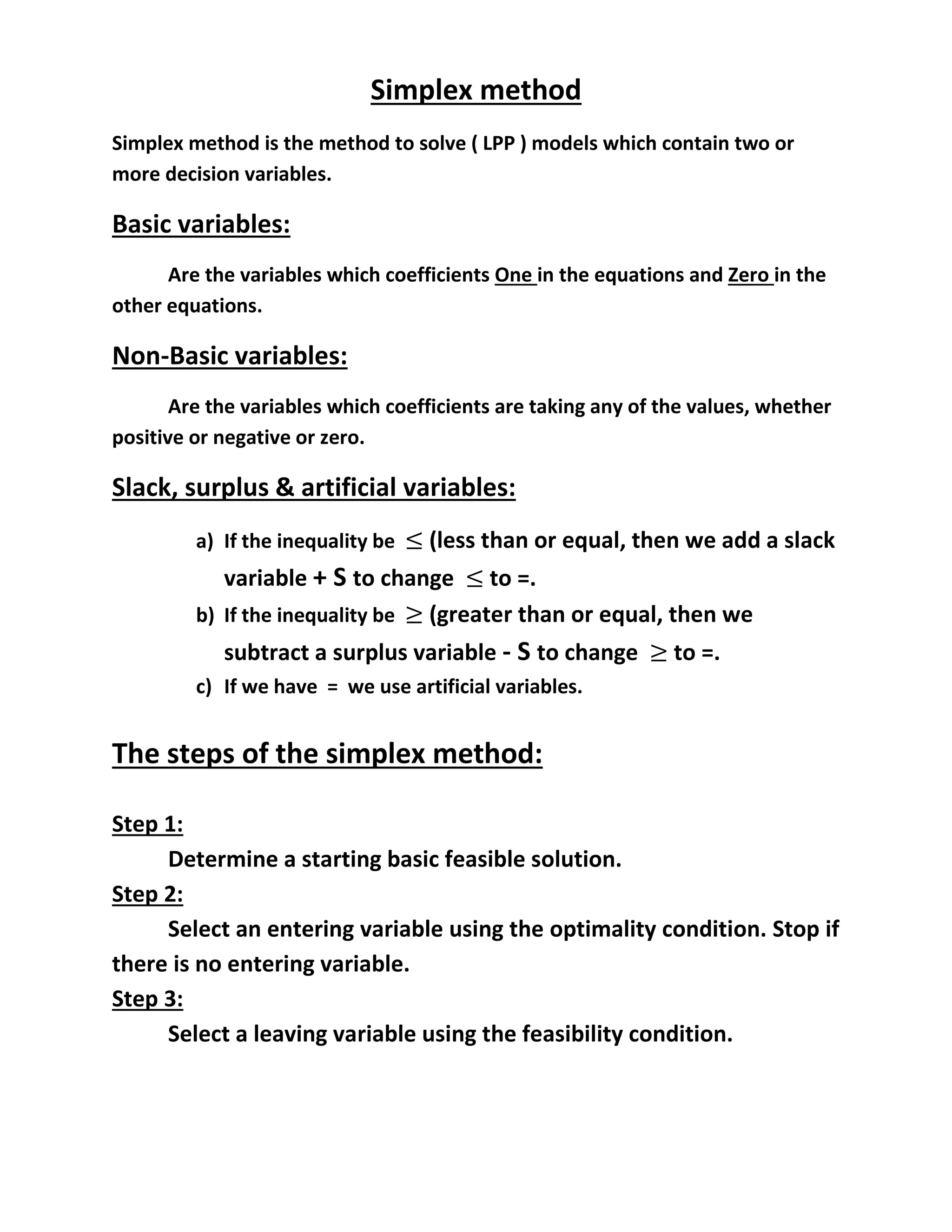
The simplex method is a technique for solving linear programming models with multiple decision variables. It involves defining basic and non-basic variables, using pivoting steps to reach an optimal solution by iterating through feasible solutions based on optimality and feasibility conditions. The document provides detailed steps and examples illustrating the application of the simplex method in solving linear programming problems.

1. Simplex method
Simplex method is the method to solve ( LPP ) models which contain two or
more decision variables.
Basic variables:
Are the variables which coefficients One in the equations and Zero in the
other equations.
Non-Basic variables:
Are the variables which coefficients are taking any of the values, whether
positive or negative or zero.
Slack, surplus & artificial variables:
a) If the inequality be (less than or equal, then we add a slack
variable + S to change to =.
b) If the inequality be (greater than or equal, then we
subtract a surplus variable - S to change to =.
c) If we have = we use artificial variables.
The steps of the simplex method:
Step 1:
Determine a starting basic feasible solution.
Step 2:
Select an entering variable using the optimality condition. Stop if
there is no entering variable.
Step 3:
Select a leaving variable using the feasibility condition.

2. Optimality condition:
The entering variable in a maximization (minimization) problem
is the non-basic variable having the most negative (positive)
coefficient in the Z-row.
The optimum is reached at the iteration where all the Z-row
coefficient of the non-basic variables are non-negative (non-positive).
Feasibility condition:
For both maximization and minimization problems the leaving
variable is the basic associated with the smallest non-negative ratio
(with strictly positive denominator).
Pivot row:
a) Replace the leaving variable in the basic column with the
entering variable.
b) New pivot row equal to current pivot row divided by pivot
element.
c) All other rows:
New row=current row - (pivot column coefficient) *new
pivot row.

3. Example 1:
Use the simplex method to solve the (LP) model:
Subject to
Solution:
Subject to

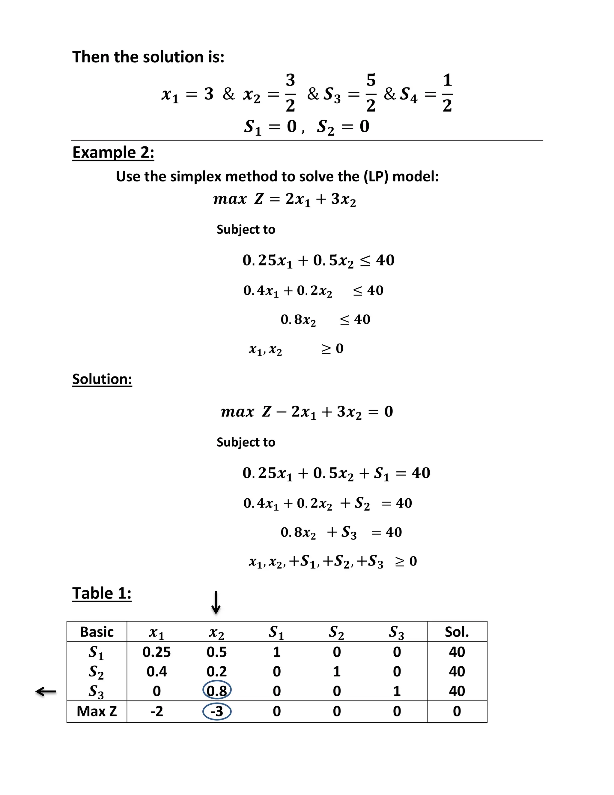
4. Table 1:
Basic Sol.
6 4 1 0 0 0 24
1 2 0 1 0 0 6
-1 1 0 0 1 0 1
0 1 0 0 0 1 2
Max Z -5 -4 0 0 0 0 0
(ignore)
(ignore)
The entering variable is and is a leaving variable.
Table 2:
 Pivot row or new -row= [current –row]
Basic Sol.
1 2/3 1/6 0 0 0 4
0 4/3 -1/6 1 0 0 2
0 5/3 1/6 0 1 0 5
0 1 0 0 0 1 2
Max Z 0 -2/3 5/6 0 0 0 20

5. - New -row=[ current –row]-(1)[ new –row]
=[1 2 0 1 0 0 6]- (1)[1 2/3 1/6 0 0 0 0 4]
=[0 4/3 -1/6 1 0 0 2]
- New -row=[ current –row]-(1)[ new –row]
=[-1 1 0 0 1 0 1]- (1)[1 2/3 1/6 0 0 0 0 4]
=[0 5/3 1/6 0 1 0 5]
- New -row=[ current –row]-(0)[ new –row]
=[0 1 0 0 0 1 2]- (0)[1 2/3 1/6 0 0 0 0 4]
=[0 1 0 0 0 1 2]
- New -row=[ current –row]-(-5)[ new –row]
=[-5 -4 0 0 0 0 0]-(-5)[1 2/3 1/6 0 0 0 0 4]
=[0 -2/3 5/6 0 0 0 20]
Now:
The entering variable is and is a leaving variable.

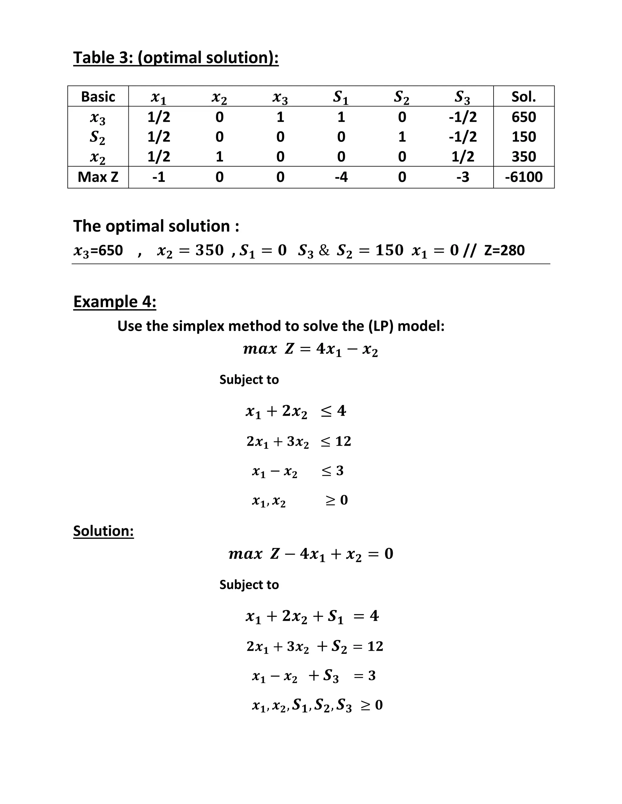
6. Table 3: (optimal solution):
 Pivot row or new -row= [current –row]
= [0 4/3 -1/6 1 0 0 2]
=[0 1 -1/8 ¾ 0 0 3/2]
- New -row=[ current –row]-(2/3)[ new –row]
=[1 2/3 1/6 0 0 0 4]- (2/3)[0 1 -1/8 ¾ 0 0 3/2]
=[1 0 ¼ -1/2 0 0 3]
- New -row=[ current –row]-(5/2)[ new –row]
=[0 5/3 1/6 0 1 0 5]-(5/3)[0 1 -1/8 ¾ 0 0 3/2]
=[0 0 3/8 -5/4 1 0 5/3]
- New -row=[ current –row]-(1)[ new –row]
=[0 1 0 0 0 1 2]-(1)[0 1 -1/8 ¾ 0 0 3/2]
=[0 0 1/8 -3/4 0 1 ½]
New -row=[ current –row]-(-2/3)[ new –row]
=[0 -2/3 5/6 0 0 0 20]-(-2/3)[0 1 -1/8 ¾ 0 0 3/2]
=[0 0 ¾ ½ 0 0 21]
Basic Sol.
1 0 1/4 -1/2 0 0 3
0 1 -1/8 3/4 0 0 3/2
0 0 3/8 -5/4 1 0 5/2
0 0 1/8 -3/4 0 1 1/2
Max Z 0 0 5/6 1/2 0 0 21

7. Then the solution is:
Example 2:
Use the simplex method to solve the (LP) model:
Subject to
Solution:
Subject to
Table 1:
Basic Sol.
0.25 0.5 1 0 0 40
0.4 0.2 0 1 0 40
0 0.8 0 0 1 40
Max Z -2 -3 0 0 0 0

8.  Pivot row or new -row= [0 0.8 0 0 1 40]
=[0 1 0 0 1.25 50]
New -row=[ current –row]-(0.5)[ new –row]
=[0.25 0.5 1 0 0 40]-(0.5)[0 1 0 0 1.25 50]
=[0 0.5 0 0 -0.625 15]
New -row=[ current –row]-(0.2)[ new –row]
=[0.4 0.2 0 1 0 40]-(0.2)[0 1 0 0 1.25 50]
[0.4 0 0 1 -0.25 30]
New -row=[ current –row]-(-3)[ new –row]
=[-2 -3 0 0 0 0]-(-3)[0 1 0 0 1.25 50]
=[-2 0 0 0 3.75 150]
Table 2:
Basic Sol.
0.25 0 1 0 -0.625 15
0.4 0 0 1 -0.25 30
0 1 0 0 1.25 50
Max Z -2 0 0 0 3.75 150

9. (ignore)
Pivot row or new -row= [0.25 0 1 0 -0.625 15]
=[1 0 4 0 -2.5 60]
New -row=[ current –row]-(0.4)[ new –row]
=[0.4 0 0 0 -0.25 30]-(0.4)[1 0 4 0 -2. 5 60]
[0 0 -1.6 0 -0.75 6]
New -row=[0 1 0 0 1.25 50]-(0)[1 0 4 0 -2. 5 60]
=[0 1 0 0 1.25 50]
New -row=[ current –row]-(-2)[ 1 0 4 0 -2.5 60]
=[-2 0 0 0 3.75 150]-(-2)[1 0 4 0 -2. 5 60]
[0 0 8 0 -1.25 270]
Table 3:
Basic Sol.
1 0 4 0 -2.5 60
0 0 -1.6 1 0.75 6
0 1 0 0 1.25 50
Max Z 0 0 8 0 -1.25 270
(ignore)

10. New -row= =[current -row] = [0 0 -1.6 0 0.75 6]
=[0 0 -2.133 0 1 8]
New -row= [1 0 4 0 -2.5 60]-(-2.5)[ 0 0 -2.133 0 1 8]
=[1 0 -1.333 0 0 80]
New -row= [0 1 0 0 1.25 50]-(-1.25)[ 0 0 -2.133 0 1 8]
=[0 1 -2.76 0 0 40]
New -row= [0 0 8 0 -1.25 270]-(-2.5)[ 0 0 -2.133 0 1 8]
=[0 0 5.33 0 0 280]
Table 3: (optimal solution):
Basic Sol.
1 0 -1.333 0 0 80
0 0 -2.133 0 1 8
0 1 -2.67 0 0 40
Max Z 0 0 5.33 0 0 280
The optimal solution :
=80 , , // Z=280
Example 3:
Use the simplex method to solve the (LP) model:
Subject to

11. Solution:
Subject to
Table 1:
New -row or -row = [1 2 0 0 0 1 700]
=[ 1 0 0 0 350]
New -row = [1 1 1 1 0 0 1000]-(1)[ 1 0 0 0 350]
=[ 0 1 1 0 - 650]
New -row = [1 1 0 0 1 0 500]-(1)[ 1 0 0 0 350]
=[ 0 0 0 1 - 150]
Basic Sol.
1 1 1 1 0 0 1000
1 1 0 0 1 0 500
1 2 0 0 1 1 700
Max Z 6 10 4 0 0 0 0

12. New -row = [6 10 4 0 0 0 0]-(10)[ 1 0 0 0 350]
=[1 0 4 0 0 - -3500]
Table 2:
(ignore)
(ignore)
New -row or -row = [ 0 1 1 0 - 650]
=[ 0 1 1 0 - 650]
New -row = [ 0 0 0 1 - 150]-(0)[ 0 1 1 0 - 650]
=[ 0 0 0 1 - 150]
New -row = [ 1 0 0 0 350]-(0)[ 0 1 1 0 - 650]
=[ 1 0 0 0 350]
New -row = [ 0 4 0 0 -5 -3500]-(4)[ 0 1 1 0 - 650]
=[-1 0 0 -4 0 -3 -6100]
Basic Sol.
1/2 0 1 1 0 -1/2 650
1/2 0 0 0 1 -1/2 150
1/2 1 0 0 0 1/2 350
Max Z 1 0 4 0 0 -5 -3500

13. Table 3: (optimal solution):
The optimal solution :
=650 , , // Z=280
Example 4:
Use the simplex method to solve the (LP) model:
Subject to
Solution:
Subject to
Basic Sol.
1/2 0 1 1 0 -1/2 650
1/2 0 0 0 1 -1/2 150
1/2 1 0 0 0 1/2 350
Max Z -1 0 0 -4 0 -3 -6100

14. Table 1:
New -row or -row = [1 -1 0 0 1 3]
=[1 -1 0 0 1 3]
New -row = [1 2 1 0 0 4]-(1)[ ]
=[0 3 1 0 -1 1]
New -row = [2 3 0 1 0 12]-(2)[ ]
=[0 5 0 1 -2 6]
New -row = [-4 1 0 0 0 0]-(-4)[ ]
=[0 -3 0 0 4 12]
Table 2:
Basic Sol.
1 2 1 0 0 4
2 3 0 1 0 12
1 -1 0 0 1 3
Max Z -4 1 0 0 0 0
Basic Sol.
0 3 1 0 -1 1
0 5 0 1 -2 6
1 -1 0 0 1 3
Max Z 0 -3 0 0 4 12

15. (ignore)
New -row or -row = [0 3 1 0 -1 1]
=[0 1 1/3 0 -1/3 1/3]
New -row = [0 5 0 1 -2 6]-(5)[ ]
=[0 0 -2/3 1 11/3 13/3]
New -row = [1 -1 0 0 1 3]-(-1)[ ]
=[1 0 1/3 0 2/3 10/3]
New -row = [0 -3 0 0 4 12]-(-3)[ ]
=[0 0 1 0 3 13]
Table 3: (optimal solution):
The optimal solution :
=10/3 , , // Z=13
Basic Sol.
0 1 1/3 0 -1/3 1/3
0 0 -2/3 1 11/3 13/3
1 0 1/3 0 2/3 10/3
Max Z 0 0 1 0 3 13

16. Example 5:
Use the simplex method to solve the (LP) model:
Subject to
Solution:
Subject to
,
Table 1:
Basic Sol.
1 2 4 1 0 0 0 2000
2 1 1 0 1 0 0 3600
1 2 2 0 0 1 0 2400
1 0 0 0 0 0 1 30
Max Z -16 -17 -10 0 0 0 0 0

17. (ignore)
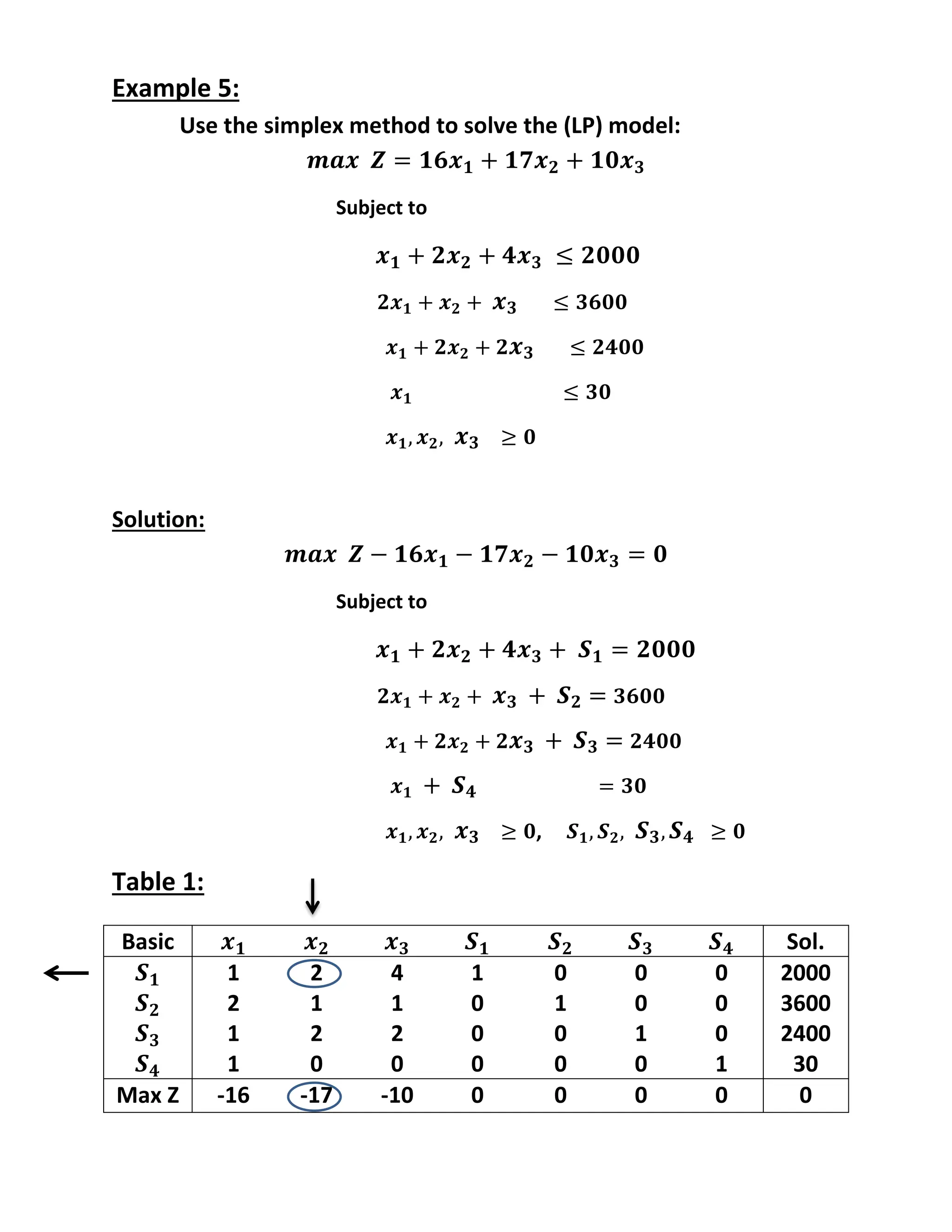
New -row or -row = [1 2 4 1 0 0 0 2000]
=[1/2 1 2 1/2 0 0 0 1000]
New -row = [2 1 1 0 1 0 0 3600]
-(1)[
=[3/2 0 -1 -1/2 1 0 0 2600]
New -row = [1 2 2 0 0 1 0 2400]
-(2)[
=[0 0 -2 -1 0 1 0 400]
New -row = [1 0 0 0 0 0 1 30]
-(0)[
=[1 0 0 0 0 0 1 30]
New -row = [-16 -17 -10 0 0 0 0 0]
-(-17)[
=[15/2 0 24 17/2 0 0 0 17000]

18. Table 2: (optimal solution):
The optimal solution :
=1000 , , /
Z=17000
Example 6:
Use the simplex method to solve the (LP) model:
Subject to
Solution:
Subject to
Basic Sol.
1/2 1 2 1/2 0 0 0 1000
3/2 0 -1 -1/2 1 0 0 2600
0 0 -2 -1 0 1 0 400
1 0 0 0 0 0 1 30
Max Z 15/2 0 24 17/2 0 0 0 17000

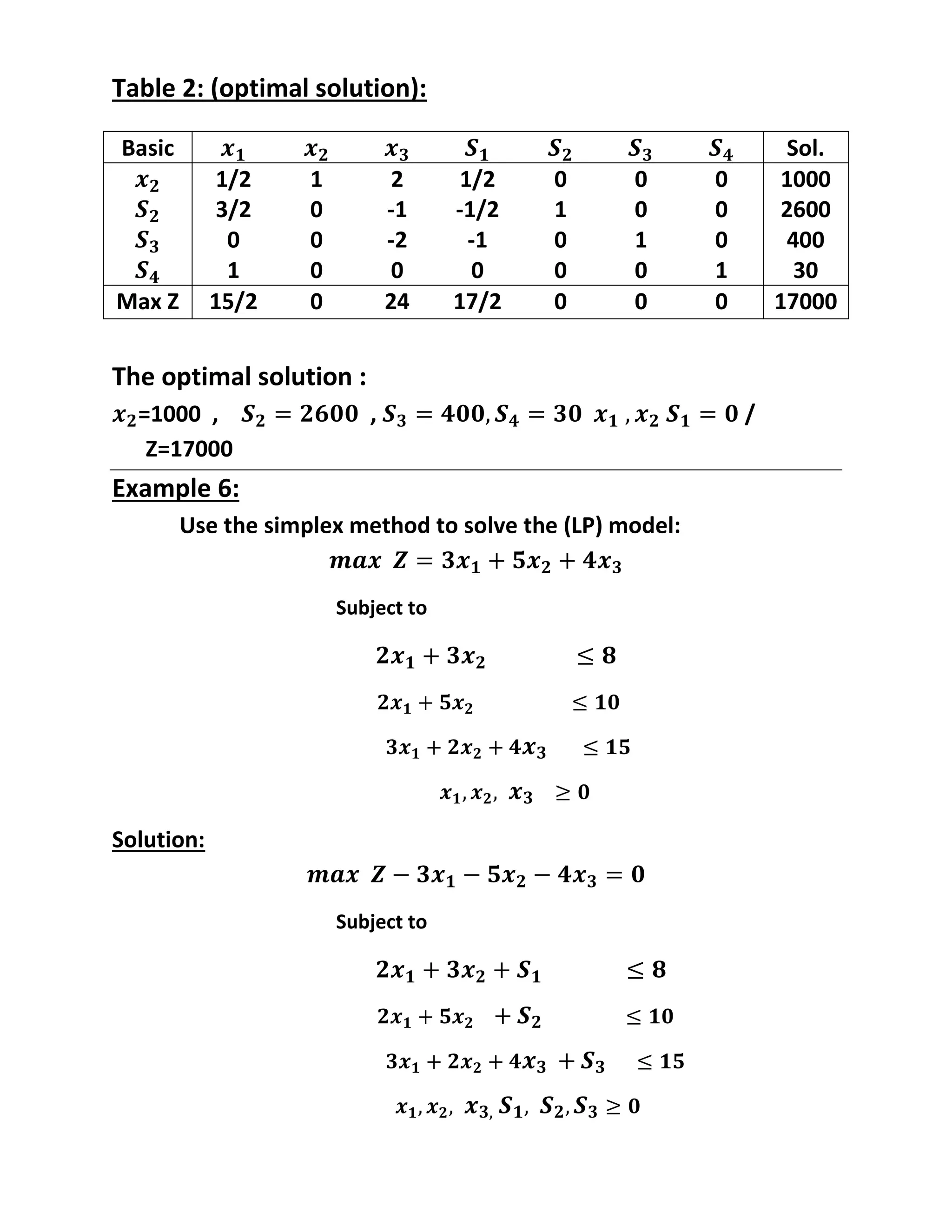
19. Table 1:
New -row or -row = [2 5 0 0 1 0 10 ]
=[2/5 1 0 0 1/5 0 2]
New -row = [2 3 0 1 0 0 8 ]
-(3)[
=[4/5 0 0 1 -3/5 0 2]
New -row = [3 2 4 0 0 1 15 ]
-(2)[
=[11/5 0 4 0 -2/5 1 11]
New -row = [-3 -5 -4 0 0 0 0 ]
-(-5)[
=[-1 0 -4 0 1 0 10]
Basic Sol.
2 3 0 1 0 0 8
2 5 0 0 1 0 10
3 2 4 0 0 1 15
Max Z -3 -5 -4 0 0 0 0

20. Table 2:
New -row or -row = [11/5 0 4 0 -2/5 1 11]
=[11/20 0 1 0 -1/10 1/4 11/4]
New -row = [4/5 0 0 1 -3/5 0 2 ]
-(0)[
=[4/5 0 0 1 -3/5 0 2]
New -row = [2/5 1 0 0 1/5 0 2 ]
New -row = [-1 0 -4 0 1 0 10 ]
-(-4)[
=[6/5 0 0 0 3/5 1 21]
Table 3: (optimal solution):
The optimal solution :
=2 ,
,
Z=21
,
Basic Sol.
4/5 0 0 1 -3/5 0 2
2/5 1 0 0 1/5 0 2
11/5 1 4 0 -2/5 1 11
Max Z -1 0 -4 0 1 0 10
Basic Sol.
4/5 0 0 1 -3/5 0 2
2/5 1 0 0 1/5 0 2
11/20 0 1 0 -1/10 1/4 11/4
Max Z 6/5 0 0 0 3/5 1 21
View publication stats
View publication stats