Download to read offline


![CBi
CBi
0 0 –M 0
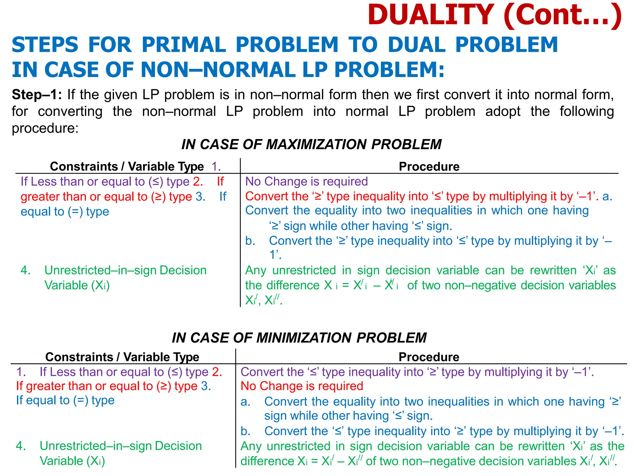
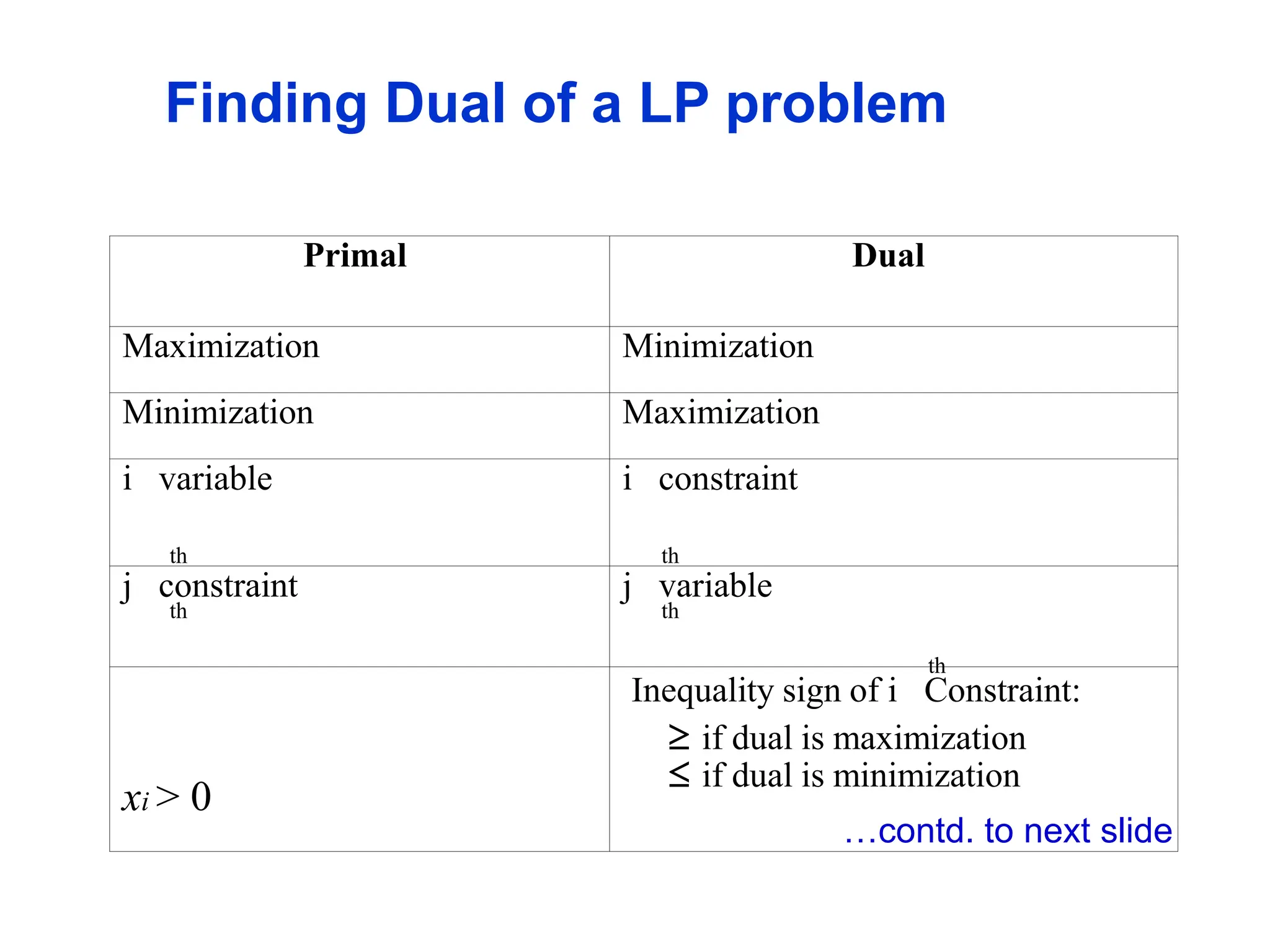
DUALITY (Cont…)
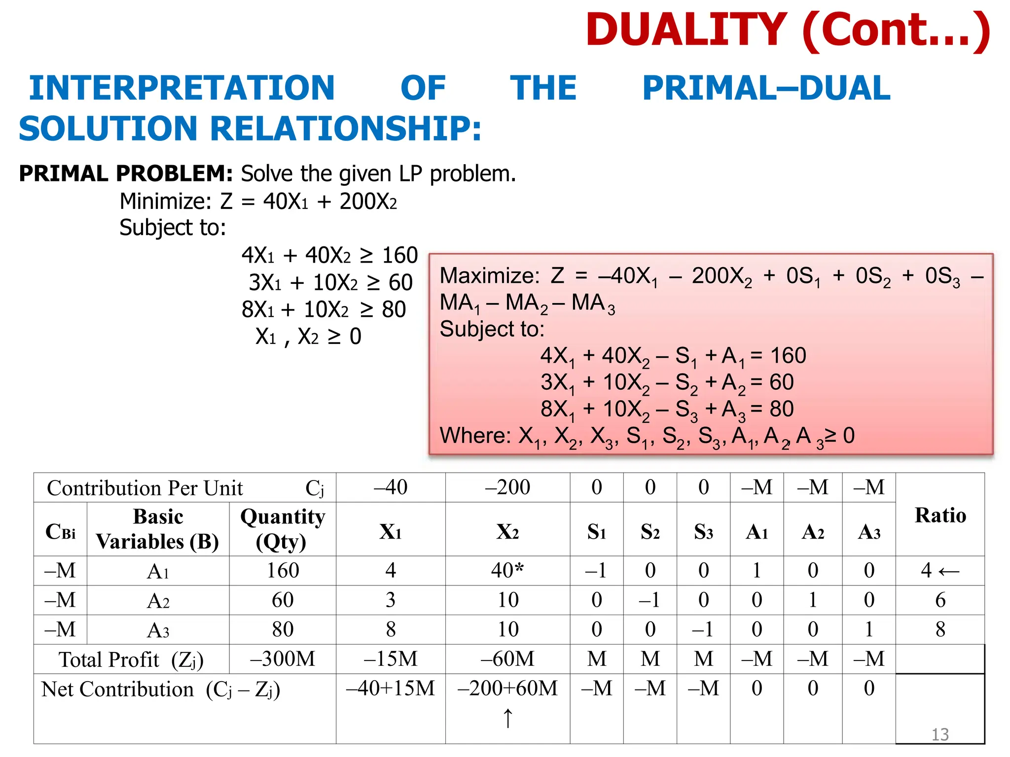
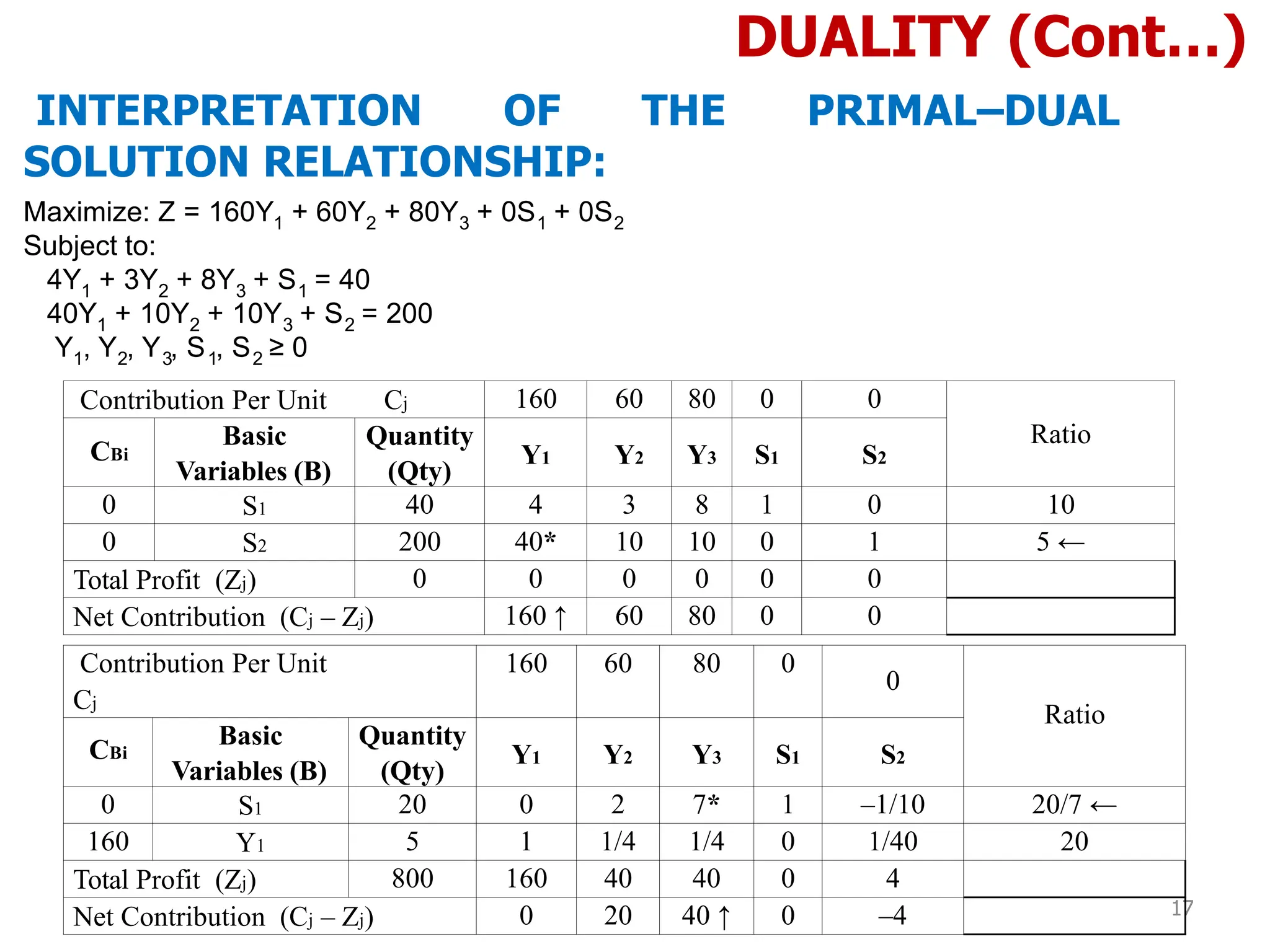
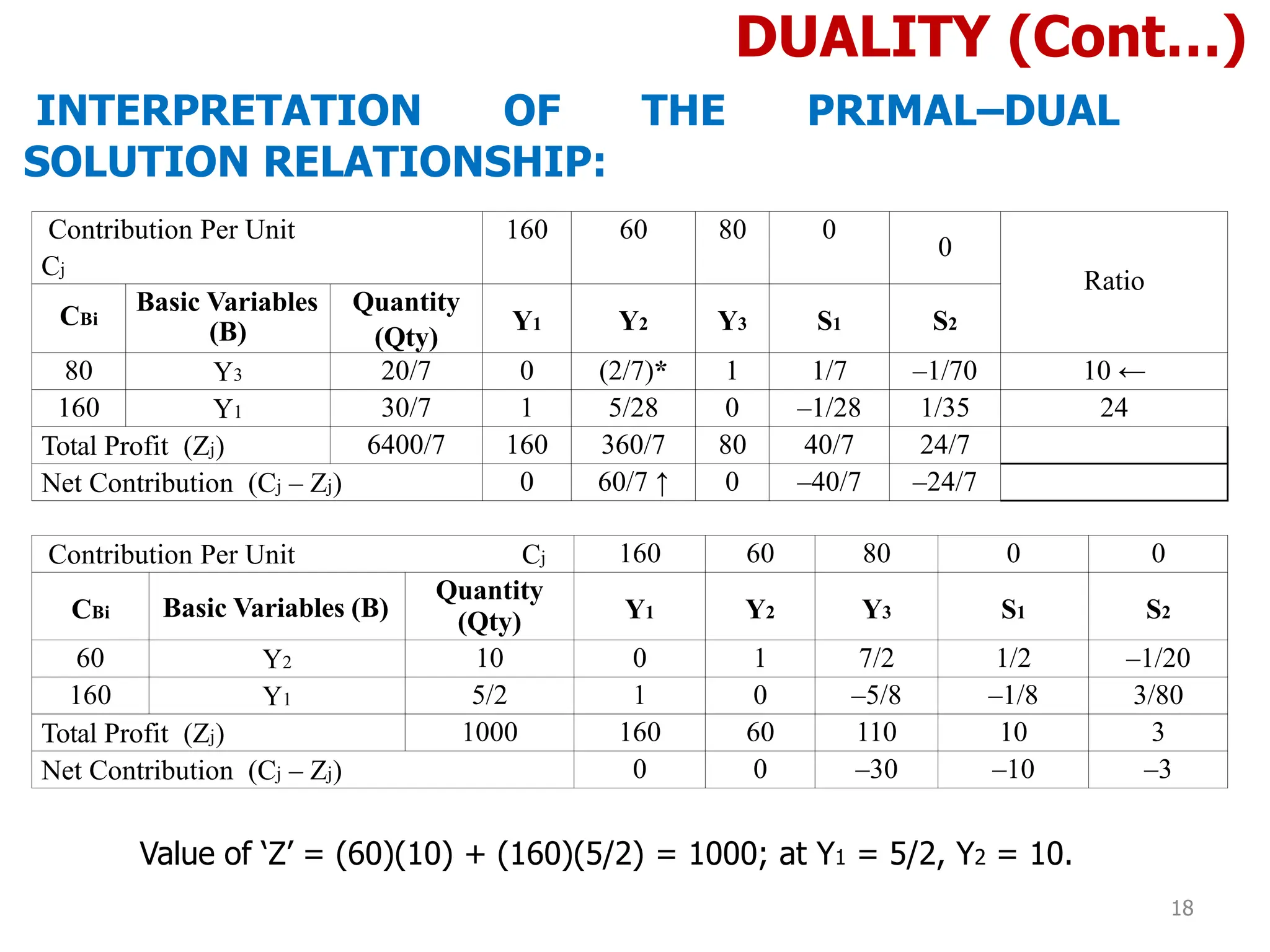
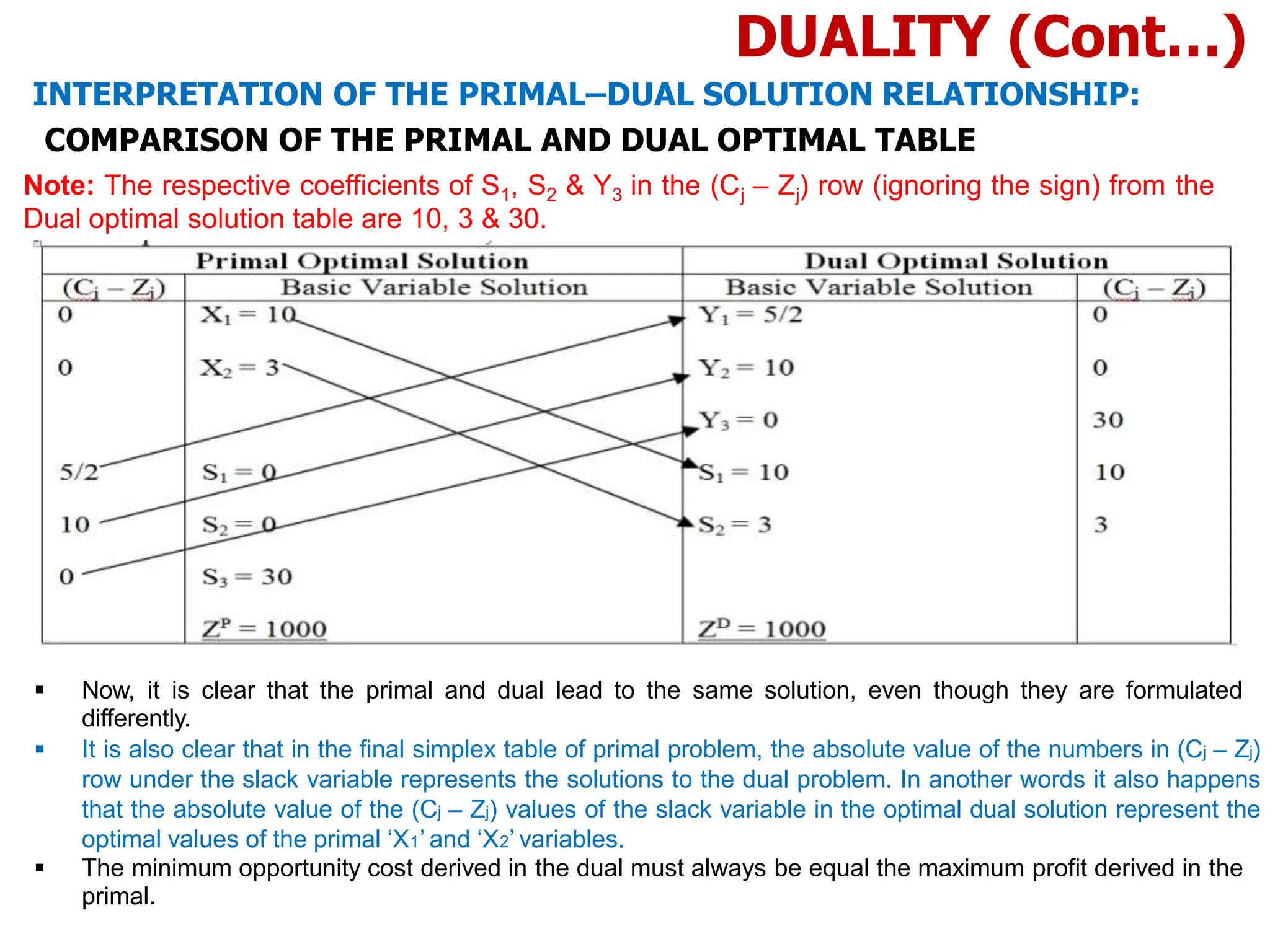
INTERPRETATION OF THE PRIMAL–DUAL
SOLUTION RELATIONSHIP:
Contribution Per Unit Cj –40 –200 0 0 0 –M –M –M
Ratio
Basic
Variables (B)
Quantity
(Qty)
X1 X2 S1 S2 S3 A1 A2 A3
–200 X2 4 1/10 1 –1/40 0 0 1/40 0 0 40
–M A2 20 2 0 1/4 –1 0 –1/4 1 0 10
–M A3 40 7* 0 1/4 0 –1 –1/4 0 1 40/7 ←
Total Profit (Zj) –800–60M –20–9M –200 5 – M/2 M M –5+M/2 –M –M
Net Contribution (C – Zj) –20+9M ↑ 0 –5+M/2 –M –M 5–3M/2 0 0
Contribution Per Unit Cj –40 –200 0 0 0 –M –M –M
Ratio
B.V.
(B)
Quantity
(Qty)
X1 X2 S1 S2 S3 A1 A2 A3
–200 X2 24/7 0 1 –1/35 0 1/70 1/35 0 –1/70 240
–M A2 60/7 0 0 5/28 –1 (2/7)* –5/28 1 –2/7 30 ←
–40 X1 40/7 1 0 1/28 0 –1/7 –1/28 0 1/7 ---
Total Profit:
(Zj)
(–6400–
60M)/7
–40 –200
(120–
5M)/28
M (20–2M)/7
(–120+
5M)/28
–M
(–20+
2M)/7
Net Contribution (Cj – Zj) (–120+
5M)/28
[(–20+
2M)/7] ↑
(120–
5M)/28
(20–
2M)/7 14](https://image.slidesharecdn.com/duelsimplexmethod-240227162153-c1bdbf1e/75/Duel-simplex-method_operations-research-pptx-9-2048.jpg)


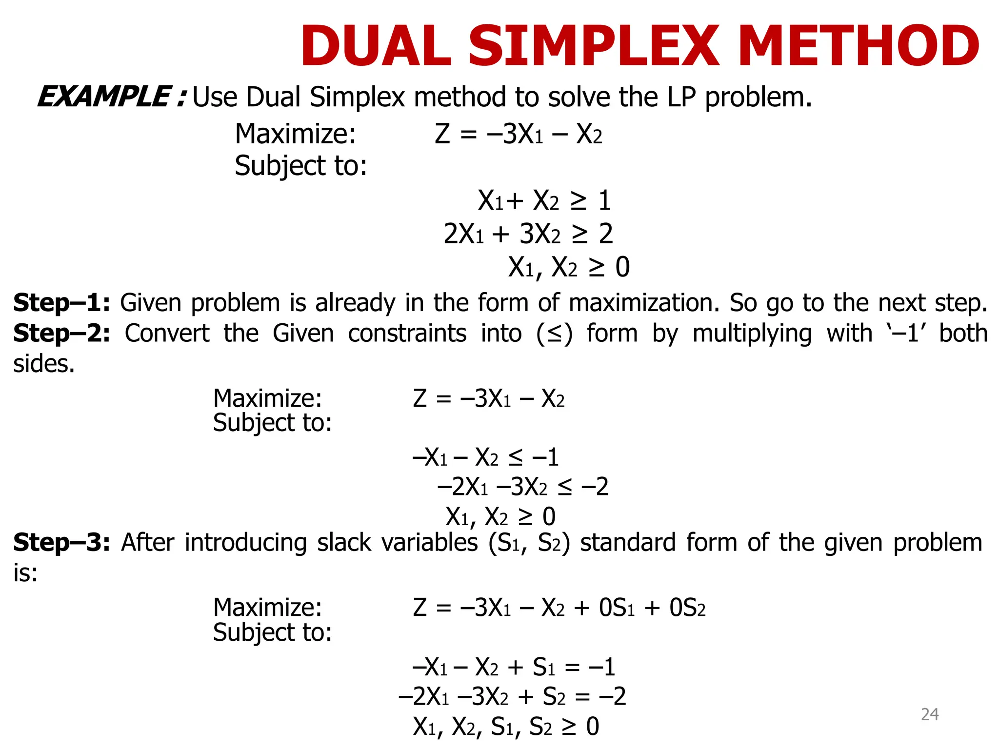
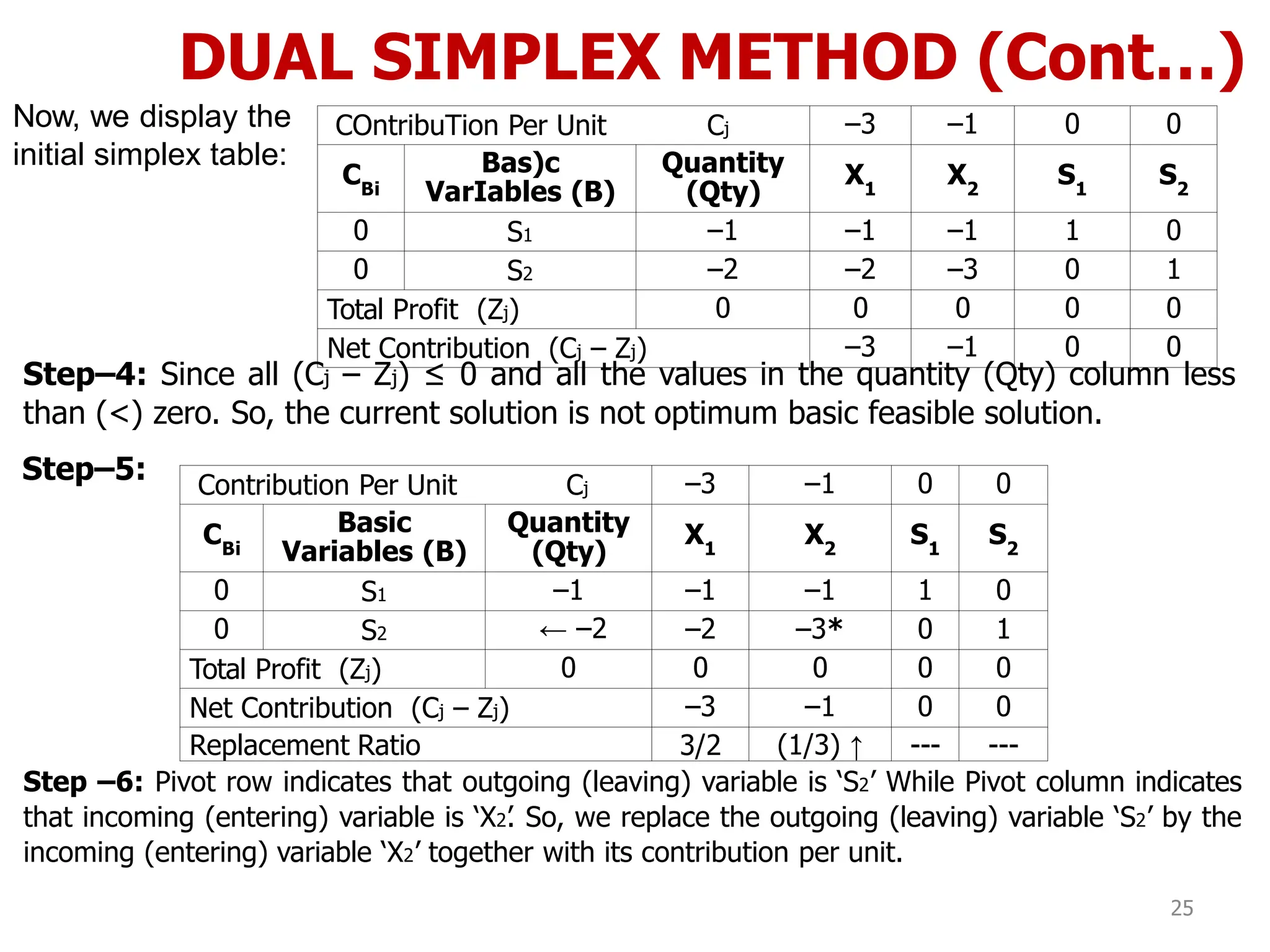
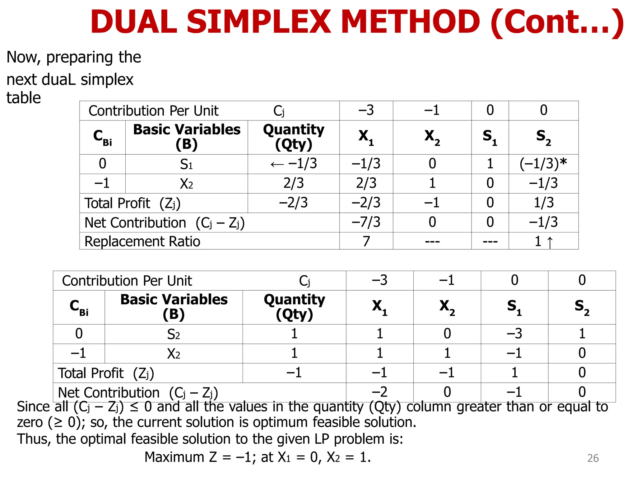
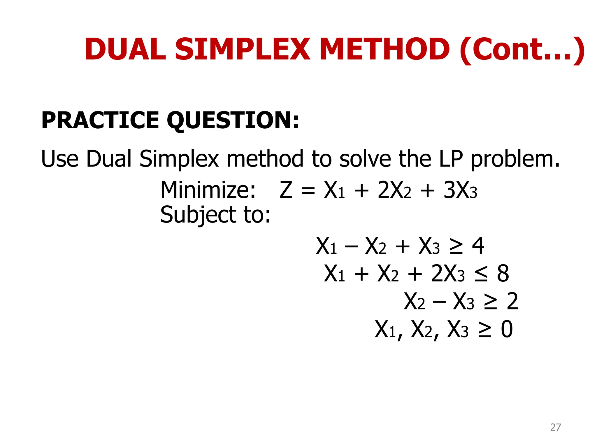

This document discusses various topics in linear programming including duality, the dual simplex method, and bounded variables linear programming problems. It provides steps to derive the dual problem from the primal problem, including converting to normal form if needed. The relationship between optimal solutions in the primal and dual problems is interpreted. Specifically, it shows that the objective function values are equal at optimality and the dual basic variables are equal to the shadow prices in the primal problem.