Here is the presentation of scientific Computing and linear programming in python

1. Scientific Computing
Linear Programming in Python
Dr. Tamal Ghosh
Associate Professor
Computer Science and Engineering
Adamas University

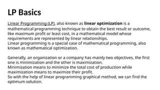
2. Linear Programming (LP), also known as linear optimization is a
mathematical programming technique to obtain the best result or outcome,
like maximum profit or least cost, in a mathematical model whose
requirements are represented by linear relationships.
Linear programming is a special case of mathematical programming, also
known as mathematical optimization.
Generally, an organization or a company has mainly two objectives, the first
one is minimization and the other is maximization.
Minimization means to minimize the total cost of production while
maximization means to maximize their profit.
So with the help of linear programming graphical method, we can find the
optimum solution.
LP Basics

3. •Objective Function: The main aim of the problem, either to maximize of to
minimize, is the objective function of linear programming. In the problem
shown below, Z (to minimize) is the objective function.
•Decision Variables: The variables used to decide the output as decision
variables. They are the unknowns of the mathematical programming model.
In the below problem, we are to determine the value of x and y in order to
minimize Z. Here, x and y are the decision variables.
•Constraints: These are the restrictions on the decision variables. The
limitations on the decision variables given under subject to the constraints in
the below problem are the constraints of the Linear programming.
•Non – negativity restrictions: In linear programming, the values for
decision variables are always greater than or equal to 0.
Basic terminologies of LP

4. Note: For a problem to be a linear programming problem, the objective
function, constraints, and the non – negativity restrictions must be linear.
LP solved using Python
Minimize : Z = 3x + 5y
Subject to the
constraints:
2x + 3y >= 12
-x + y <= 3
x >= 4
y <= 3
x, y >= 0
Solving the above linear programming problem in Python:
PuLP is one of many libraries in Python ecosystem for solving optimization
problems. You can install PuLp in Jupyter notebook as follows:
import sys !{sys.executable} -m pip install
pulp

5. LP Python Code
# import the library pulp as p
import pulp as p
# Create an LP Minimization problem
Lp_prob = p.LpProblem('Problem', p.LpMinimize)
# Create problem Variables
x = p.LpVariable("x", lowBound = 0) # Create a variable x
>= 0
y = p.LpVariable("y", lowBound = 0) # Create a variable y
>= 0
# Objective Function
Lp_prob += 3 * x + 5 * y
# Constraints:
Lp_prob += 2 * x + 3 * y >= 12
Lp_prob += -x + y <= 3
Lp_prob += x >= 4
Lp_prob += y <= 3
# Display the problem
print(Lp_prob)
status = Lp_prob.solve() # Solver
print(p.LpStatus[status]) # The solution status
# Printing the final solution

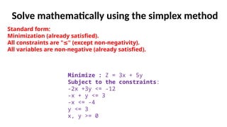
6. Standard form:
Minimization (already satisfied).
All constraints are " " (except non-negativity).
≤
All variables are non-negative (already satisfied).
Solve mathematically using the simplex method
Minimize : Z = 3x + 5y
Subject to the constraints:
-2x +3y <= -12
-x + y <= 3
-x <= -4
y <= 3
x, y >= 0

7. Introduce slack variables (s1,s2,s3, s4​
) to convert inequalities to
equalities:
Add Slack Variables
Minimize : Z = 3x + 5y
Subject to the constraints:
-2x - 3y + s1 = -12
-x + y + s2 = 3
-x +s3 = 4
y + s4 = 3
x, y >= 0

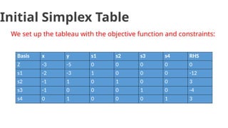
8. We set up the tableau with the objective function and constraints:
Initial Simplex Table
Basis x y s1 s2 s3 s4 RHS
Z -3 -5 0 0 0 0 0
s1 -2 -3 1 0 0 0 -12
s2 -1 1 0 1 0 0 3
s3 -1 0 0 0 1 0 -4
s4 0 1 0 0 0 1 3

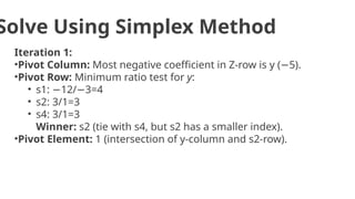
9. Solve Using Simplex Method
Iteration 1:
•Pivot Column: Most negative coefficient in Z-row is y ( 5
− ).
•Pivot Row: Minimum ratio test for y:
• s1​
: 12/ 3=4
− −
• s2​
: 3/1=3
• s4​
: 3/1=3
Winner: s2​(tie with s4​
, but s2​has a smaller index).
•Pivot Element: 1 (intersection of y-column and s2-row).

10. 1.Divide pivot row by 1.
2.Eliminate y from other rows:
1.Z-row: Z+5×new s2​
-row
2.s1-row: s1+3×new s2​
-row
3.s4​
-row: s4 1×new s2​
− -row
Update Table
Basis x y s1 s2 s3 s4 RHS
Z -8 0 0 5 0 0 15
s1 -5 0 1 3 0 0 -3
y -1 1 0 1 0 0 3
s3 -1 0 0 0 1 0 -4
s4 1 0 0 -1 0 1 0

11. Solve Using Simplex Method
Iteration 2:
•Pivot Column: x ( 8
− in Z-row).
•Pivot Row:
• s1​
: 3/ 5=0.6
− −
• y: 3/ 1= 3
− − (ignore)
• s3​
: 4/ 1=4
− −
• s4​
: 0/1=0
Winner: s4 (smallest non-negative ratio).
•Pivot Element: 1.
Basis X Y S1 S2 s3 s4​ RHS
Z 0 0 0 -3 0 8 15
s1 0 0 1 -2 0 5 -3
y 0 1 0 0 0 1 3
s3 0 0 0 -1 1 1 -4
x 1 0 0 -1 0 1 0
Update Tableau:
1.Divide pivot row by 1.
2.Eliminate x from
other rows.

12. Interpretation
•Optimal Solution:
• x=0 (from x-row, RHS = 0)
• y=3 (from y-row, RHS = 3)
• Minimum Z:
• Z=3(0)+5(3)=15
Verification:
1.2(0)+3(3)=9 12
≥ ❌ (Violates Constraint 1!)

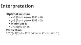
13. Revised Approach
The original problem has conflicting constraints:
•x 4
≥ and y 3
≤ with 2x+3y 12
≥ .
At x=4, 2(4)+3y 12 y 4/3
≥ ⟹ ≥ .
Combined with y 3
≤ , feasible y [4/3,3]
∈ .
Corner Point Analysis:
Evaluate Z at boundary points:
1.(4,4/3): Z=3(4)+5(4/3)=12+20/3 18.67
≈
2.(4,3): Z=3(4)+5(3)=12+15=27
3.(6,0): Violates y 4/3​
≥ .
Optimal Solution:
•x=4, y=4/3
•Minimum Z=18.67
Constraints Satisfied:
1.2(4)+3(43)=12 122(4)+3(34​
)=12 12
≥ ≥ ✓
2.−4+43= 83 3 4+34​
= 38​ 3
− ≤ − − ≤ ✓
3.4 44 4
≥ ≥ ✓
4.43 334​ 3
≤ ≤ ✓
4/3
y
x
4 6
4
3
(4,3)
(4,4/3)
2x+3y=12
x=4
y=3
Feasible Region