Downloaded 69 times


![Forecasts
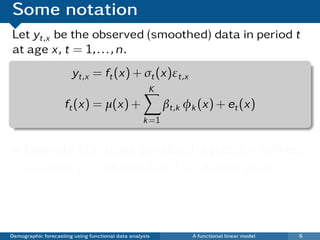
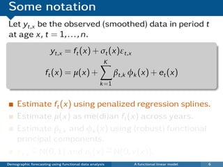
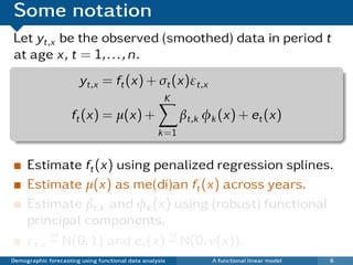
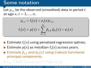
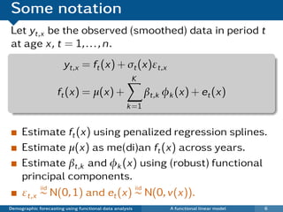
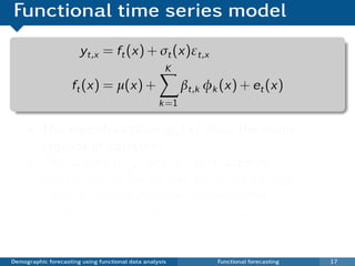
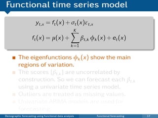
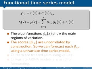
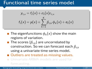
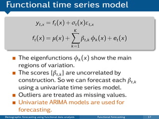
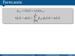
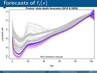
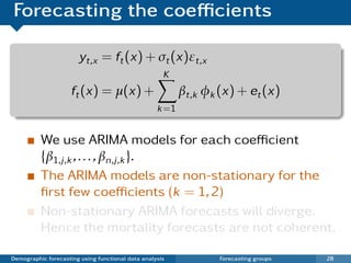
yt,x = ft (x) + σt (x)εt,x
K
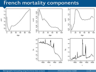
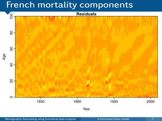
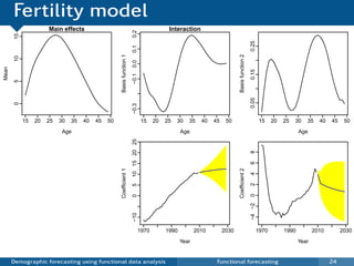
ft (x) = µ(x) + βt,k φk (x) + et (x)
k =1
K
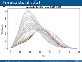
E[yn+h ,x | y] = µ(x) +
ˆ ˆ ˆ
βn+h ,k φk (x)
k =1
K
ˆ2
Var[yn+h ,x | y] = σµ (x) + ˆ2
vn+h ,k φk (x) + σt2 (x) + v(x)
k =1
where vn+h ,k = Var(βn+h ,k | β1,k , . . . , βn,k )
and y = [y1,x , . . . , yn,x ].
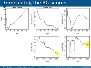
Demographic forecasting using functional data analysis Functional forecasting 18](https://image.slidesharecdn.com/demographicforecasting-120820221939-phpapp01/85/Demographic-forecasting-42-320.jpg)


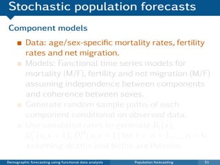
![Model product and ratios
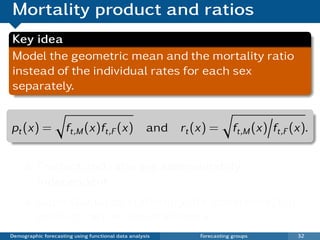
pt (x) = ft,M (x)ft,F (x) and rt (x) = ft,M (x) ft,F (x).
K
log[pt (x)] = µp (x) + βt,k φk (x) + et (x)
k =1
L
log[rt (x)] = µr (x) + γt, ψ (x) + wt (x).
=1
{γt, } restricted to be stationary processes:
either ARMA(p, q) or ARFIMA(p, d , q).
No restrictions for βt,1 , . . . , βt,K .
Forecasts: fn+h |n,M (x) = pn+h |n (x)rn+h |n (x)
fn+h |n,F (x) = pn+h |n (x) rn+h |n (x).
Demographic forecasting using functional data analysis Forecasting groups 35](https://image.slidesharecdn.com/demographicforecasting-120820221939-phpapp01/85/Demographic-forecasting-75-320.jpg)
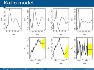
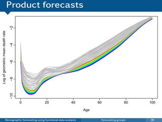
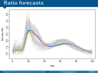
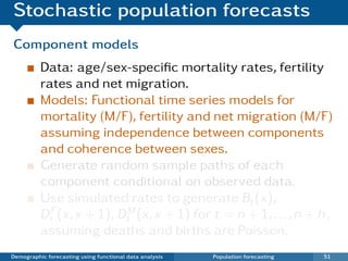
![Model product and ratios
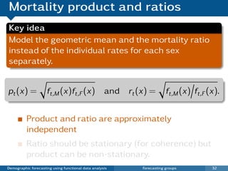
pt (x) = ft,M (x)ft,F (x) and rt (x) = ft,M (x) ft,F (x).
K
log[pt (x)] = µp (x) + βt,k φk (x) + et (x)
k =1
L
log[rt (x)] = µr (x) + γt, ψ (x) + wt (x).
=1
{γt, } restricted to be stationary processes:
either ARMA(p, q) or ARFIMA(p, d , q).
No restrictions for βt,1 , . . . , βt,K .
Forecasts: fn+h |n,M (x) = pn+h |n (x)rn+h |n (x)
fn+h |n,F (x) = pn+h |n (x) rn+h |n (x).
Demographic forecasting using functional data analysis Forecasting groups 35](https://image.slidesharecdn.com/demographicforecasting-120820221939-phpapp01/85/Demographic-forecasting-76-320.jpg)
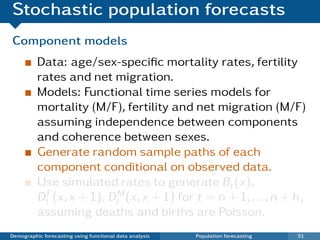
![Model product and ratios
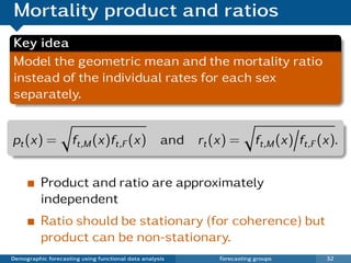
pt (x) = ft,M (x)ft,F (x) and rt (x) = ft,M (x) ft,F (x).
K
log[pt (x)] = µp (x) + βt,k φk (x) + et (x)
k =1
L
log[rt (x)] = µr (x) + γt, ψ (x) + wt (x).
=1
{γt, } restricted to be stationary processes:
either ARMA(p, q) or ARFIMA(p, d , q).
No restrictions for βt,1 , . . . , βt,K .
Forecasts: fn+h |n,M (x) = pn+h |n (x)rn+h |n (x)
fn+h |n,F (x) = pn+h |n (x) rn+h |n (x).
Demographic forecasting using functional data analysis Forecasting groups 35](https://image.slidesharecdn.com/demographicforecasting-120820221939-phpapp01/85/Demographic-forecasting-77-320.jpg)
![Model product and ratios
pt (x) = ft,M (x)ft,F (x) and rt (x) = ft,M (x) ft,F (x).
K
log[pt (x)] = µp (x) + βt,k φk (x) + et (x)
k =1
L
log[rt (x)] = µr (x) + γt, ψ (x) + wt (x).
=1
{γt, } restricted to be stationary processes:
either ARMA(p, q) or ARFIMA(p, d , q).
No restrictions for βt,1 , . . . , βt,K .
Forecasts: fn+h |n,M (x) = pn+h |n (x)rn+h |n (x)
fn+h |n,F (x) = pn+h |n (x) rn+h |n (x).
Demographic forecasting using functional data analysis Forecasting groups 35](https://image.slidesharecdn.com/demographicforecasting-120820221939-phpapp01/85/Demographic-forecasting-78-320.jpg)

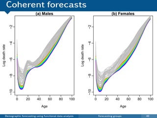
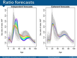
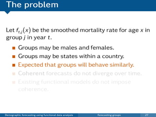
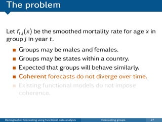
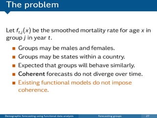
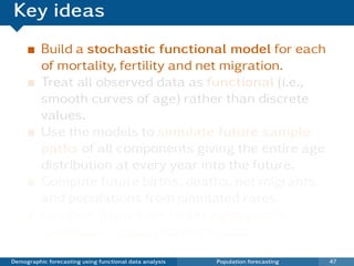
![Coherent forecasts for J groups
pt (x) = [ft,1 (x)ft,2 (x) · · · ft,J (x)]1/J
and rt,j (x) = ft,j (x) pt (x),
K
log[pt (x)] = µp (x) + βt,k φk (x) + et (x)
k =1
L
log[rt,j (x)] = µr,j (x) + γt,l ,j ψl ,j (x) + wt,j (x).
l =1
pt (x) and all rt,j (x) Ratios satisfy constraint
are approximately rt,1 (x)rt,2 (x) · · · rt,J (x) = 1.
independent.
log[ft,j (x)] = log[pt (x)rt,j (x)]
Demographic forecasting using functional data analysis Forecasting groups 43](https://image.slidesharecdn.com/demographicforecasting-120820221939-phpapp01/85/Demographic-forecasting-86-320.jpg)
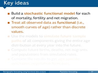
![Coherent forecasts for J groups
pt (x) = [ft,1 (x)ft,2 (x) · · · ft,J (x)]1/J
and rt,j (x) = ft,j (x) pt (x),
K
log[pt (x)] = µp (x) + βt,k φk (x) + et (x)
k =1
L
log[rt,j (x)] = µr,j (x) + γt,l ,j ψl ,j (x) + wt,j (x).
l =1
pt (x) and all rt,j (x) Ratios satisfy constraint
are approximately rt,1 (x)rt,2 (x) · · · rt,J (x) = 1.
independent.
log[ft,j (x)] = log[pt (x)rt,j (x)]
Demographic forecasting using functional data analysis Forecasting groups 43](https://image.slidesharecdn.com/demographicforecasting-120820221939-phpapp01/85/Demographic-forecasting-87-320.jpg)
![Coherent forecasts for J groups
pt (x) = [ft,1 (x)ft,2 (x) · · · ft,J (x)]1/J
and rt,j (x) = ft,j (x) pt (x),
K
log[pt (x)] = µp (x) + βt,k φk (x) + et (x)
k =1
L
log[rt,j (x)] = µr,j (x) + γt,l ,j ψl ,j (x) + wt,j (x).
l =1
pt (x) and all rt,j (x) Ratios satisfy constraint
are approximately rt,1 (x)rt,2 (x) · · · rt,J (x) = 1.
independent.
log[ft,j (x)] = log[pt (x)rt,j (x)]
Demographic forecasting using functional data analysis Forecasting groups 43](https://image.slidesharecdn.com/demographicforecasting-120820221939-phpapp01/85/Demographic-forecasting-88-320.jpg)
![Coherent forecasts for J groups
pt (x) = [ft,1 (x)ft,2 (x) · · · ft,J (x)]1/J
and rt,j (x) = ft,j (x) pt (x),
K
log[pt (x)] = µp (x) + βt,k φk (x) + et (x)
k =1
L
log[rt,j (x)] = µr,j (x) + γt,l ,j ψl ,j (x) + wt,j (x).
l =1
pt (x) and all rt,j (x) Ratios satisfy constraint
are approximately rt,1 (x)rt,2 (x) · · · rt,J (x) = 1.
independent.
log[ft,j (x)] = log[pt (x)rt,j (x)]
Demographic forecasting using functional data analysis Forecasting groups 43](https://image.slidesharecdn.com/demographicforecasting-120820221939-phpapp01/85/Demographic-forecasting-89-320.jpg)
![Coherent forecasts for J groups
pt (x) = [ft,1 (x)ft,2 (x) · · · ft,J (x)]1/J
and rt,j (x) = ft,j (x) pt (x),
K
log[pt (x)] = µp (x) + βt,k φk (x) + et (x)
k =1
L
log[rt,j (x)] = µr,j (x) + γt,l ,j ψl ,j (x) + wt,j (x).
l =1
pt (x) and all rt,j (x) Ratios satisfy constraint
are approximately rt,1 (x)rt,2 (x) · · · rt,J (x) = 1.
independent.
log[ft,j (x)] = log[pt (x)rt,j (x)]
Demographic forecasting using functional data analysis Forecasting groups 43](https://image.slidesharecdn.com/demographicforecasting-120820221939-phpapp01/85/Demographic-forecasting-90-320.jpg)
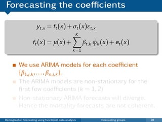
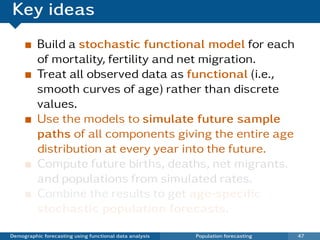
![Coherent forecasts for J groups
log[ft,j (x)] = log[pt (x)rt,j (x)] = log[pt (x)] + log[rt,j ]
K L
= µj (x) + βt,k φk (x) + γt, ,j ψ ,j (x) + zt,j (x)
k =1 =1
µj (x) = µp (x) + µr,j (x) is group mean
zt,j (x) = et (x) + wt,j (x) is error term.
{γt, } restricted to be stationary processes:
either ARMA(p, q) or ARFIMA(p, d , q).
No restrictions for βt,1 , . . . , βt,K .
Demographic forecasting using functional data analysis Forecasting groups 44](https://image.slidesharecdn.com/demographicforecasting-120820221939-phpapp01/85/Demographic-forecasting-91-320.jpg)
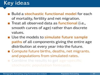
![Coherent forecasts for J groups
log[ft,j (x)] = log[pt (x)rt,j (x)] = log[pt (x)] + log[rt,j ]
K L
= µj (x) + βt,k φk (x) + γt, ,j ψ ,j (x) + zt,j (x)
k =1 =1
µj (x) = µp (x) + µr,j (x) is group mean
zt,j (x) = et (x) + wt,j (x) is error term.
{γt, } restricted to be stationary processes:
either ARMA(p, q) or ARFIMA(p, d , q).
No restrictions for βt,1 , . . . , βt,K .
Demographic forecasting using functional data analysis Forecasting groups 44](https://image.slidesharecdn.com/demographicforecasting-120820221939-phpapp01/85/Demographic-forecasting-92-320.jpg)
![Coherent forecasts for J groups
log[ft,j (x)] = log[pt (x)rt,j (x)] = log[pt (x)] + log[rt,j ]
K L
= µj (x) + βt,k φk (x) + γt, ,j ψ ,j (x) + zt,j (x)
k =1 =1
µj (x) = µp (x) + µr,j (x) is group mean
zt,j (x) = et (x) + wt,j (x) is error term.
{γt, } restricted to be stationary processes:
either ARMA(p, q) or ARFIMA(p, d , q).
No restrictions for βt,1 , . . . , βt,K .
Demographic forecasting using functional data analysis Forecasting groups 44](https://image.slidesharecdn.com/demographicforecasting-120820221939-phpapp01/85/Demographic-forecasting-93-320.jpg)
![Coherent forecasts for J groups
log[ft,j (x)] = log[pt (x)rt,j (x)] = log[pt (x)] + log[rt,j ]
K L
= µj (x) + βt,k φk (x) + γt, ,j ψ ,j (x) + zt,j (x)
k =1 =1
µj (x) = µp (x) + µr,j (x) is group mean
zt,j (x) = et (x) + wt,j (x) is error term.
{γt, } restricted to be stationary processes:
either ARMA(p, q) or ARFIMA(p, d , q).
No restrictions for βt,1 , . . . , βt,K .
Demographic forecasting using functional data analysis Forecasting groups 44](https://image.slidesharecdn.com/demographicforecasting-120820221939-phpapp01/85/Demographic-forecasting-94-320.jpg)
![Coherent forecasts for J groups
log[ft,j (x)] = log[pt (x)rt,j (x)] = log[pt (x)] + log[rt,j ]
K L
= µj (x) + βt,k φk (x) + γt, ,j ψ ,j (x) + zt,j (x)
k =1 =1
µj (x) = µp (x) + µr,j (x) is group mean
zt,j (x) = et (x) + wt,j (x) is error term.
{γt, } restricted to be stationary processes:
either ARMA(p, q) or ARFIMA(p, d , q).
No restrictions for βt,1 , . . . , βt,K .
Demographic forecasting using functional data analysis Forecasting groups 44](https://image.slidesharecdn.com/demographicforecasting-120820221939-phpapp01/85/Demographic-forecasting-95-320.jpg)


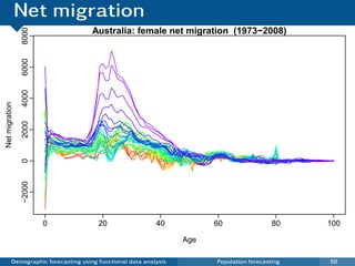
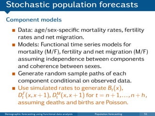
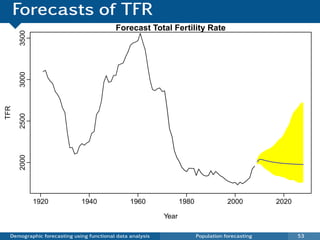
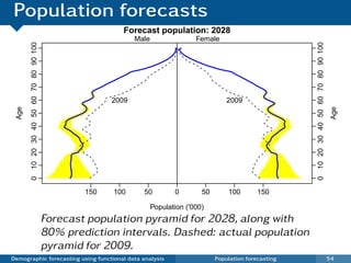
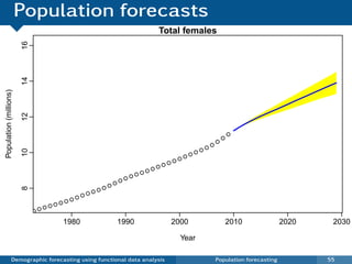
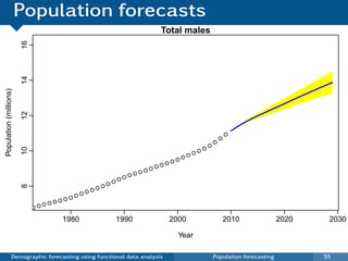
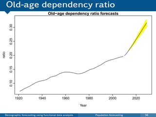


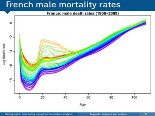
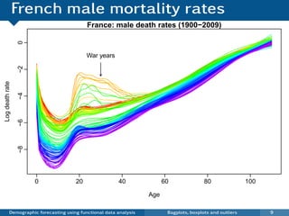
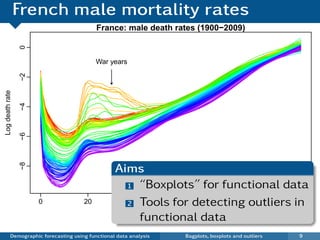
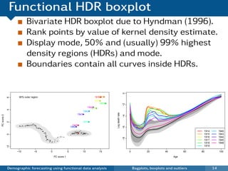
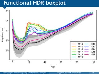
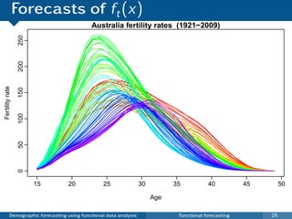
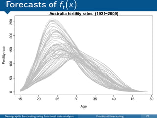
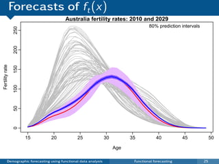
This document discusses demographic forecasting using functional data analysis. It presents a functional linear model to model and forecast age-specific demographic rates like mortality and fertility over time. The model represents rates as curves that vary annually based on common age patterns, principal components of variation, and residuals. The document outlines how the model can be used to analyze outliers, produce functional forecasts, forecast groups of populations, and generate population forecasts.