05 Random Variables

Stat310
Discrete random variables

Hadley Wickham
Tuesday, 26 January 2010

Homework
• Don’t forget to pledge!
• Model answers up v. soon, and on track
to get your homeworks back on
Thursday.
• Homework help session Tuesday &
Wednesday 4-5pm. Details on webpage.
• Will be other extra credit opportunities


Data visualisation
mini course
Feb 13 (Saturday). 10am - 3pm.
http://www.ece.rice.edu/ece/
datavis2010.html
The applied side of statistics - getting
data and ﬁguring out what is going on.
No maths, lots of graphics and
programming


1. Independence example
2. Random variables
1. Bernoulli
2. Binomial
3. Mean and variance


Are the wearing glasses and
wearing hat events independent?

21 Dennis Washingtons in total

Calculations
P(glasses) = 9 / 21
P(hat) = 9 / 21
P(glasses and hat) = 3 / 21 = 0.14
P(glasses) P(hat) = 9 / 49 = 0.18
Wearing a glasses and hat together is
(slightly) less likely than we’d expect if they
were independent.


Deﬁnitions
A random variable is a random experiment
with a numeric sample space. Usually given
a capital letter like X, Y or Z.
(More formally a random variable is a function
that converts outcomes from a random
experiment into numbers)
The space (or support) of a random variable
is the range of the function (cf. sample space)


Definitions

If the size of the support is finite or
countably infinite, then the random
variable is discrete.
If the size of the support is uncountably
infinite, then the random variable is
continuous.


pmf/pdf
Every random experiment has a probability
function.
Every discrete random variable as
probability mass function (pmf).
Every continuous random variable has
probability density function (pdf).
Different ways of deﬁning the function that
says how likely each outcome is.


This week: discrete
Next week: continuous
This diverges from the book, but I think
it’s easier to work with one set of
mathematical tools at a time


Notation
Normally call pmf f
If we have multiple rv’s and want to make
clear which pmf belongs to which rv, we
write:
fX(x) fY(y) fZ(z) for X, Y, Z
f1(x) f2(x) f3(3) for X1, X2, X3


P (X = xi ) = f (xi )

P (a X b) = f (xi )
xi ∈(a,b)

To be a pmf, f must satisfy:

f (xi ) = 1
xi ∈S
f (xi ) ≥ 0, ∀ xi ∈ S


x f(x) x f(x) x f(x)
-1 0.3 10 -0.1 1 0.35
0 0.3 20 0.9 2 0.25
2 0.3 30 0.2 3 0.2
4 0.1
x f(x) x f(x)
5 0.1
5 1 10 0.1
20 0.9
30 0.2

Notation
Can give pmf in two ways:
• List of numbers (for small n)
• Function (for large n)
These are equivalent!
Also useful to display visually.


a) b)
0.8
1.0

0.6 0.8

0.6
0.4
f(x)

f(x)
0.4
0.2
0.2

0.0 0.0
1.0 1.5 2.0 2.5 3.0 1.0 1.5 2.0 2.5 3.0
x x

c) d)
0.5
0.4
0.4

0.3 0.3

0.2
f(x)

f(x)
0.2
0.1
0.1
0.0

0.0 −0.1
1 2 3 4 5 1 2 3 4 5
x x

Distributions
In practice, many real problems can be
approximated with just a few different
families of pmf/pdfs. These are called
distributions.
A distribution has parameters which control
how it acts. If a random variable has a
named distribution, then we write it as:
X ~ DistributionName(parameters)


Bernoulli distribution
Single binary event: either happens (with
probability p) or doesn’t happen.
Let X be a random variable that takes the
value 1 if the event happens, 0 otherwise.
Then X ~ Bernoulli(p)
f(1) = P(X = 1) = p
f(0) = ?


Wait, is that a pmf?


Binomial distribution

n independent Bernoulli trials with the
same probability of success. Let X be the
number of successes.
Then we say X ~ Binomial(n, p)
P(X = x) = f(x) = ??


Wait, is that a pmf?
Random mathematical fact.
Need to check the two conditions.
First easy, second a bit harder.

(If I ever give you a random mathematical
fact you can expect to use it. Main
challenge is recognising where it is needed)


Example
Let X be the number of babies that a
woman has in the next 5 years. Assume
the chance of having a baby in a given year
is a constant 10%.
What additional assumption do we need to
use the binomial distribution? Is it
reasonable?
What is f(0)? What is f(1)? What is P(X 0)?


Mean variance
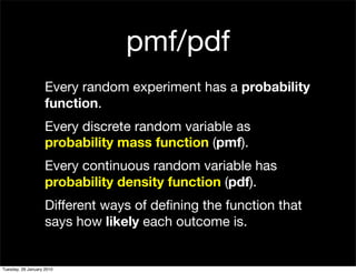
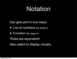
Mean summarises the “middle” of the
distribution. Variance summarise the
“spread” of the distribution.
Mean = E(X) = “Sum” of all outcomes,
weighted by their probability.
Variance = Var(X) = E[ (X - E[X])2) ] =
expected squared distance from mean


Intuition for mean

Imagine the number line as a beam with
weights of f(x) at position x. The balance
point is the mean.


Example

Assume 95% of you have 0 stds. 4% of
you have 1 std. 1% have 2 stds. What is
the expected number of stds?

http://www.cdc.gov/mmwr/preview/mmwrhtml/ss5806a1.htm

Mean of a binomial
random variable
For named distributions we can usually
work out the mean (and variance) as
functions of the parameters.
This is typically a little tricky, but once
we’ve done it, we can use a simple
formula every time we see that
distribution.


Another way

http://www.wolframalpha.com/input/?
i=sum_(x%3D0)^(n)+(x+n!+/+(x!+(n-x)!)
+p^x+(1-p)^(n-x))


05 Random Variables

More Related Content

What's hot

Viewers also liked

Similar to 05 Random Variables

More from Hadley Wickham

Recently uploaded

05 Random Variables