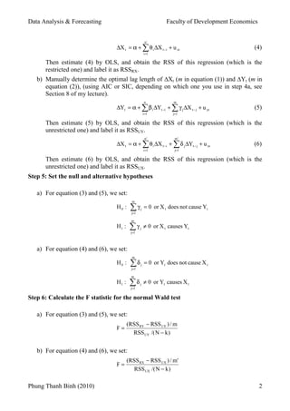
The document describes the standard Granger causality test procedure for determining whether changes in one time series (Xt) can help forecast changes in another (Yt). [1] The test involves estimating a VAR model with the two time series and their lags, then comparing the restricted and unrestricted models to calculate an F-statistic. [2] If the F-statistic exceeds the critical value, the null hypothesis that Xt does not help forecast Yt (or vice versa) is rejected, indicating Granger causality between the two time series. [3] The test results help explain the relationship between the changes in the two time series by determining the direction of causality (if any

1. Data Analysis & Forecasting Faculty of Development Economics
TIME SERIES ANALYSIS
STANDARD/STATIC GRANGER CAUSALITY
1. THE MODEL
The Standard/Static Granger Causality test for the of two stationary variables ∆Yt and ∆Xt,
involves as a first step the estimation of the following VAR model:
n m
∆Yt = α + ∑ β i ∆Yt −i + ∑ γ j ∆X t − j + u yt (1)
i =1 j=1
n m
∆X t = α + ∑ θ i ∆X t −i + ∑ δ j ∆Yt − j + u xt (2)
i =1 j=1
Important note: In practice, the lag n and m in equation (1) and (2) might be not the same.
However, if you perform the test in Eviews, the routine VAR model assumes that both n
and m in both equation are the same. This kind of selection can lead to model
mispecification. Therefore, we should manually determine the optimal lag length for them
(see the guide in step 4 below).
2. TEST PROCEDURE
Suppose we have Yt and Xt are nonstationary.
THE STANDER GRANGER CAUSALITY is performed as follows:
Step 1: Testing for the unit root of Yt and Xt
(using either DF, ADF, or PP tests)
Suppose the test results indicate that both Yt and Xt are I(1).
Step 2: Testing for cointegration between Yt and Xt
(usually use Engle-Granger (EG) or Johansen approach)
If the test results indicate that Yt and Xt are not cointegrated, we have only one choice of
Standard Version of Granger Causality. Conversely, if Yt and Xt are cointegrated, we can
apply either Standard or ECM Version of Granger Causality, depending on our research
objectives.
Step 3: Taking the first differences of Yt and Xt (i.e., Yt and Xt)
Step 4: Determining the optimal lag length of Yt and Xt
a) Automatically determine the optimal lag length of ∆Yt and ∆Xt in their AR models
(using AIC or SIC, see Section 8 of my lecture).
n
∆Yt = α + ∑ β i ∆Yt −i + u yt (3)
i =1
Then estimate (3) by OLS, and obtain the RSS of this regression (which is the
restricted one) and label it as RSSRY.
Phung Thanh Binh (2010) 1

2. Data Analysis & Forecasting Faculty of Development Economics
n'
∆X t = α + ∑ θ i ∆X t −i + u xt (4)
i =1
Then estimate (4) by OLS, and obtain the RSS of this regression (which is the
restricted one) and label it as RSSRX.
b) Manually determine the optimal lag length of ∆Xt (m in equation (1)) and ∆Yt (m in
equation (2)), (using AIC or SIC, depending on which one you use in step 4a, see
Section 8 of my lecture).
n m
∆Yt = α + ∑ β i ∆Yt −i + ∑ γ j ∆X t − j + u yt (5)
i =1 j=1
Then estimate (5) by OLS, and obtain the RSS of this regression (which is the
unrestricted one) and label it as RSSUY.
n' m'
∆X t = α + ∑ θ i ∆X t −i + ∑ δ j ∆Yt − j + u xt (6)
i =1 j=1
Then estimate (6) by OLS, and obtain the RSS of this regression (which is the
unrestricted one) and label it as RSSUX.
Step 5: Set the null and alternative hypotheses
a) For equation (3) and (5), we set:
m
H0 : ∑γ
j=1
j = 0 or X t does not cause Yt
m
H1 : ∑γ
j=1
j ≠ 0 or X t causes Yt
a) For equation (4) and (6), we set:
m
H0 : ∑δ
j=1
j = 0 or Yt does not cause X t
m
H1 : ∑δ
j=1
j ≠ 0 or Yt causes X t
Step 6: Calculate the F statistic for the normal Wald test
a) For equation (3) and (5), we set:
(RSS RY − RSS UY ) / m
F=
RSS UY /( N − k )
b) For equation (4) and (6), we set:
(RSS RX − RSS UX ) / m'
F=
RSS UX /( N − k )
Phung Thanh Binh (2010) 2

3. Data Analysis & Forecasting Faculty of Development Economics
If the computed F value exceeds the critical F value, reject the null hypothesis and conclude
that Xt causes Yt, or Yt causes Xt.
Question: How to explain the test results?
Phung Thanh Binh (2010) 3