Download as PDF, PPTX

.
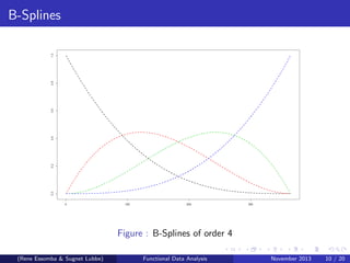
In R: create.bspline.basis(rangeval,nbasis,norder,...) (fda package)
(Rene Essomba & Sugnet Lubbe) Functional Data Analysis November 2013 9 / 20](https://image.slidesharecdn.com/sasaslidesver2-140717024015-phpapp01/85/Introduction-to-Functional-Data-Analysis-9-320.jpg)
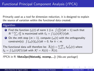
![Functional Principal Component Analysis (f PCA)
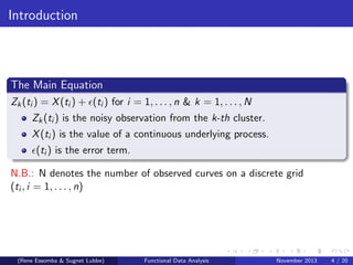
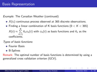
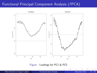
Example (Canadian Weather)
R> temp.svd <- fdata2pc(tempdat.fdata, ncomp=3)
R> norm.fdata(temp.svd$rotation[1:2])
[,1]
[1,] 0.9976567
[2,] 0.9980333
# With 3 components that explained 98.56% of the
variability of explicative variables.
# Variability for each component (%): PC1 88.03 PC2 8.47
PC3 2.06
(Rene Essomba & Sugnet Lubbe) Functional Data Analysis November 2013 16 / 20](https://image.slidesharecdn.com/sasaslidesver2-140717024015-phpapp01/85/Introduction-to-Functional-Data-Analysis-16-320.jpg)
![Functional Linear Regression Model (f LRM)
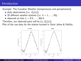
Consider the following functional linear regression models:
Functional response with multivariate covariates:
yi (t) = β1(t)xi1 + · · · + βp(t)xip + i (t); i = 1, . . . , N
Scalar response with functional covariates:
yi = α +
T
0
p
j=1
βj (s)xij (s)ds + i ; i = 1, . . . , N; s ∈ [0, T].
Functional response with functional covariates:
yi (t) = α(t) +
T
0
p
j=1
βj (t, s)xij (s)ds + i (t); i = 1, . . . , N; s ∈ [0, T].
(Rene Essomba & Sugnet Lubbe) Functional Data Analysis November 2013 18 / 20](https://image.slidesharecdn.com/sasaslidesver2-140717024015-phpapp01/85/Introduction-to-Functional-Data-Analysis-18-320.jpg)

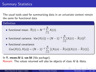
This document provides an introduction to Functional Data Analysis (FDA), highlighting key concepts such as basis representation, summary statistics, functional principal component analysis, and functional linear regression models. It covers the application of FDA through examples, specifically using R packages for data analysis. The document outlines methodologies for expressing functional data and analyzing variation, as well as practical examples, particularly related to Canadian weather data.