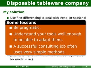
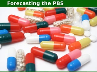
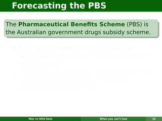
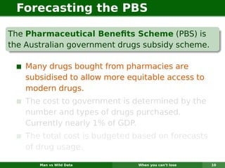
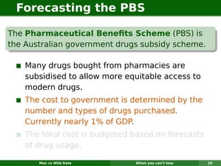
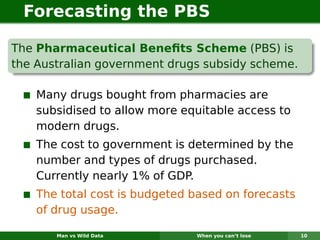
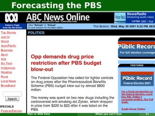
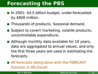
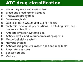
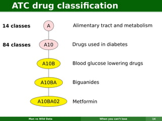
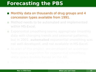
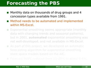
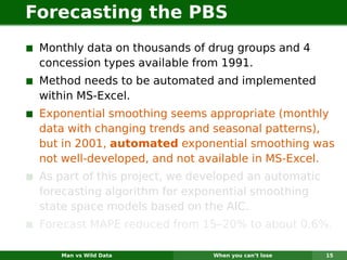
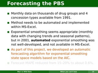
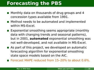
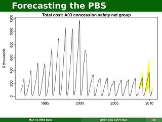
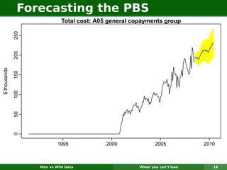
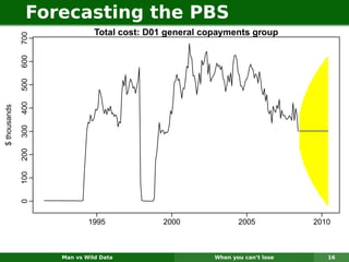
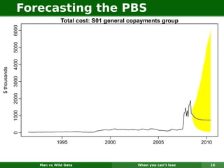
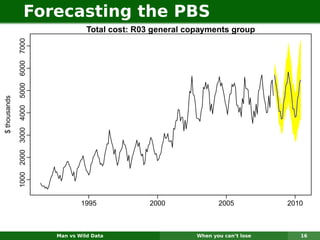
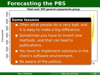
The document describes forecasting expenditures for Australia's Pharmaceutical Benefits Scheme (PBS). PBS forecasts billions in drug subsidies annually using simple Excel methods. The author developed an automated exponential smoothing algorithm in Excel, reducing forecast errors from 15-20% to 0.6%. Monthly data on thousands of drug groups was used to automatically select exponential smoothing models based on AIC.
Automatic algorithms for time series forecastingRob Hyndman
Many applications require a large number of time series to be forecast completely automatically. For example, manufacturing companies often require weekly forecasts of demand for thousands of products at dozens of locations in order to plan distribution and maintain suitable inventory stocks. In these circumstances, it is not feasible for time series models to be developed for each series by an experienced analyst. Instead, an automatic forecasting algorithm is required.
In addition to providing automatic forecasts when required, these algorithms also provide high quality benchmarks that can be used when developing more specific and specialized forecasting models.
I will describe some algorithms for automatically forecasting univariate time series that have been developed over the last 20 years. The role of forecasting competitions in comparing the forecast accuracy of these algorithms will also be discussed.
Ways to evaluate a machine learning model’s performanceMala Deep Upadhaya
Some of the ways to evaluate a machine learning model’s performance.
In Summary:
Confusion matrix: Representation of the True positives (TP), False positives (FP), True negatives (TN), False negatives (FN)in a matrix format.
Accuracy: Worse happens when classes are imbalanced.
Precision: Find the answer of How much the model is right when it says it is right!
Recall: Find the answer of How many extra right ones, the model missed when it showed the right ones!
Specificity: Like Recall but the shift is on the negative instances.
F1 score: Is the harmonic mean of precision and recall so the higher the F1 score, the better.
Precision-Recall or PR curve: Curve between precision and recall for various threshold values.
ROC curve: Graph is plotted against TPR and FPR for various threshold values.
Reduction in customer complaints - Mortgage IndustryPranov Mishra
The project aims at analysis of Customer Complaints/Inquiries received by a US based mortgage (loan) servicing company..
The goal of the project is building a predictive model using the identified significant
contributors and coming up with recommendations for changes which will lead to
1. Reducing Re-work
2. Reducing Operational Cost
3. Improve Customer Satisfaction
4. Improve company preparedness to respond to customer.
Three models were built - Logistic Regression, Random Forest and Gradient Boosting. It was seen that the accuracy, auc (Area under the curve), sensitivity and specificity improved drastically as the model complexity increased from simple to complex.
Logistic regression was not generalizing well to a non-linear data. So the model was suffering from both bias and variance. Random Forest is an ensemble technique in itself and helps with reducing variance to a great extent. Gradient Boosting, with its sequential learning ability, helps reduce the bias. The results from both random forest and gradient boosting did not differ by much. This is confirming the bias-variance trade-off concept which states that complex models will do well on non-linear data as the inflexible simple models will have high bias and can have high variance.
Additionally, a lift chart was built which gives a Cumulative lift of 133% in the first four deciles
Forecasting Techniques - Data Science SG Kai Xin Thia
Presentation by Kai Xin on techniques learnt from Forecasting - Principles and Practice book: www.otexts.org/fpp
Cover techniques like Seasonal and Trend decomposition using Loess (STL), Holts-Winters, ARIMA etc. R code adapted from the book is available at:
https://github.com/thiakx/Forecasting_DSSG
This Machine Learning Algorithms presentation will help you learn you what machine learning is, and the various ways in which you can use machine learning to solve a problem. At the end, you will see a demo on linear regression, logistic regression, decision tree and random forest. This Machine Learning Algorithms presentation is designed for beginners to make them understand how to implement the different Machine Learning Algorithms.
Below topics are covered in this Machine Learning Algorithms Presentation:
1. Real world applications of Machine Learning
2. What is Machine Learning?
3. Processes involved in Machine Learning
4. Type of Machine Learning Algorithms
5. Popular Algorithms with a hands-on demo
- Linear regression
- Logistic regression
- Decision tree and Random forest
- N Nearest neighbor
What is Machine Learning: Machine Learning is an application of Artificial Intelligence (AI) that provides systems the ability to automatically learn and improve from experience without being explicitly programmed.
- - - - - - - -
About Simplilearn Machine Learning course:
A form of artificial intelligence, Machine Learning is revolutionizing the world of computing as well as all people’s digital interactions. Machine Learning powers such innovative automated technologies as recommendation engines, facial recognition, fraud protection and even self-driving cars.This Machine Learning course prepares engineers, data scientists and other professionals with knowledge and hands-on skills required for certification and job competency in Machine Learning.
- - - - - - -
Why learn Machine Learning?
Machine Learning is taking over the world- and with that, there is a growing need among companies for professionals to know the ins and outs of Machine Learning
The Machine Learning market size is expected to grow from USD 1.03 Billion in 2016 to USD 8.81 Billion by 2022, at a Compound Annual Growth Rate (CAGR) of 44.1% during the forecast period.
- - - - - -
What skills will you learn from this Machine Learning course?
By the end of this Machine Learning course, you will be able to:
1. Master the concepts of supervised, unsupervised and reinforcement learning concepts and modeling.
2. Gain practical mastery over principles, algorithms, and applications of Machine Learning through a hands-on approach which includes working on 28 projects and one capstone project.
3. Acquire thorough knowledge of the mathematical and heuristic aspects of Machine Learning.
4. Understand the concepts and operation of support vector machines, kernel SVM, naive Bayes, decision tree classifier, random forest classifier, logistic regression, K-nearest neighbors, K-means clustering and more.
5. Be able to model a wide variety of robust Machine Learning algorithms including deep learning, clustering, and recommendation systems
- - - - - - -
Alleviating Privacy Attacks Using Causal ModelsAmit Sharma
Machine learning models, especially deep neural networks have been shown to reveal membership information of inputs in the training data. Such membership inference attacks are a serious privacy concern, for example, patients providing medical records to build a model that detects HIV would not want their identity to be leaked. Further, we show that the attack accuracy amplifies when the model is used to predict samples that come from a different distribution than the training set, which is often the case in real world applications. Therefore, we propose the use of causal learning approaches where a model learns the causal relationship between the input features and the outcome. An ideal causal model is known to be invariant to the training distribution and hence generalizes well to shifts between samples from the same distribution and across different distributions. First, we prove that models learned using causal structure provide stronger differential privacy guarantees than associational models under reasonable assumptions. Next, we show that causal models trained on sufficiently large samples are robust to membership inference attacks across different distributions of datasets and those trained on smaller sample sizes always have lower attack accuracy than corresponding associational models. Finally, we confirm our theoretical claims with experimental evaluation on 4 moderately complex Bayesian network datasets and a colored MNIST image dataset. Associational models exhibit upto 80\% attack accuracy under different test distributions and sample sizes whereas causal models exhibit attack accuracy close to a random guess. Our results confirm the value of the generalizability of causal models in reducing susceptibility to privacy attacks. Paper available at https://arxiv.org/abs/1909.12732
This is an elaborate presentation on how to predict employee attrition using various machine learning models. This presentation will take you through the process of statistical model building using Python.
Module 4: Model Selection and EvaluationSara Hooker
Delta Analytics is a 501(c)3 non-profit in the Bay Area. We believe that data is powerful, and that anybody should be able to harness it for change. Our teaching fellows partner with schools and organizations worldwide to work with students excited about the power of data to do good.
Welcome to the course! These modules will teach you the fundamental building blocks and the theory necessary to be a responsible machine learning practitioner in your own community. Each module focuses on accessible examples designed to teach you about good practices and the powerful (yet surprisingly simple) algorithms we use to model data.
To learn more about our mission or provide feedback, take a look at www.deltanalytics.org.
Causal Inference in Data Science and Machine LearningBill Liu
Event: https://learn.xnextcon.com/event/eventdetails/W20042010
Video: https://www.youtube.com/channel/UCj09XsAWj-RF9kY4UvBJh_A
Modern machine learning techniques are able to learn highly complex associations from data, which has led to amazing progress in computer vision, NLP, and other predictive tasks. However, there are limitations to inference from purely probabilistic or associational information. Without understanding causal relationships, ML models are unable to provide actionable recommendations, perform poorly in new, but related environments, and suffer from a lack of interpretability.
In this talk, I provide an introduction to the field of causal inference, discuss its importance in addressing some of the current limitations in machine learning, and provide some real-world examples from my experience as a data scientist at Brex.
Dowhy: An end-to-end library for causal inferenceAmit Sharma
In addition to efficient statistical estimators of a treatment's effect, successful application of causal inference requires specifying assumptions about the mechanisms underlying observed data and testing whether they are valid, and to what extent. However, most libraries for causal inference focus only on the task of providing powerful statistical estimators. We describe DoWhy, an open-source Python library that is built with causal assumptions as its first-class citizens, based on the formal framework of causal graphs to specify and test causal assumptions. DoWhy presents an API for the four steps common to any causal analysis---1) modeling the data using a causal graph and structural assumptions, 2) identifying whether the desired effect is estimable under the causal model, 3) estimating the effect using statistical estimators, and finally 4) refuting the obtained estimate through robustness checks and sensitivity analyses. In particular, DoWhy implements a number of robustness checks including placebo tests, bootstrap tests, and tests for unoberved confounding. DoWhy is an extensible library that supports interoperability with other implementations, such as EconML and CausalML for the the estimation step.
Prescriptive Analytics: A Hands-on Introduction to Getting Actionable Insight...Barton Poulson
Need to know the best course of action for your company? You need prescriptive analytics, an approach to analysis that mines data for actionable insights and helps you improve your company’s reach and ROI. Prescriptive analytics is more than predictive modeling; it gives valuable conditional outcomes and cause-and-effect insight. In this workshop, we’ll explore the logic of prescriptive analytics and use Excel and R to conduct simple “what-if” simulations, cross-lagged designs, optimization models, and robust quasi-experimental analyses. You’ll leave with a collection of tools that will help you intelligently choose the best path to find new value for your company.
Statistics for UX Professionals - Jessica CameronUser Vision
Are you looking to expand your research toolkit to include some quantitative methods, such as survey research or A/B testing? Have you been asked to collect some usability metrics, but aren’t sure how best to go about that? Or do you just want to be more aware of all of the UX research possibilities? If your answer to any of those questions is yes, then this session is for you.
You may know that without statistics, you won’t know if A is really better than B, if users are truly more satisfied with your new site than with your old one, or which changes to your site have actually impacted conversion rates. However, statistics can also help you figure out how to report satisfaction and other metrics you collect during usability tests. And they’re essential for making sense of the results of quantitative usability tests.
This session will focus on the statistical concepts that are most useful for UX researchers. It won’t make you a quant, but it will give you a good grounding in quantitative methods and reporting. (For example, you will learn what a margin of error is, how to report quantitative data collected during a usability test - and how not to - and how many people you really need to fill out a survey.)
Forecasting using data workshop slides for the Deliver conference in Winnipeg October 2016. This session introduces practical exercises for probabilistic forecasting. http://www.prdcdeliver.com
This lecture covers the main items that plague all of the machine learning algorithms, namely Bias and Variance. Besides, the lecture demonstrates underfitting, overfitting, and generalization. there are two questions you should have an answer after completion of this lecture: how do you know that your algorithm is subjected to overfitting, and how do you overcome this phenomenon. regularization is the main hot topic that is covered in this lecture
Traditional randomized experiments allow us to determine the overall causal impact of a treatment program (e.g. marketing, medical, social, education, political). Uplift modeling (also known as true lift, net lift, incremental lift) takes a further step to identify individuals who are truly positively influenced by a treatment through data mining / machine learning. This technique allows us to identify the “persuadables” and thus optimize target selection in order to maximize treatment benefits. This important subfield of data mining/data science/business analytics has gained significant attention in areas such as personalized marketing, personalized medicine, and political election with plenty of publications and presentations appeared in recent years from both industry practitioners and academics.
In this workshop, I will introduce the concept of Uplift, review existing methods, contrast with the traditional approach, and introduce a new method that can be implemented with standard software. A method and metrics for model assessment will be recommended. Our discussion will include new approaches to handling a general situation where only observational data are available, i.e. without randomized experiments, using techniques from causal inference. Additionally, an integrated modeling approach for uplift and direct response (where it can be identified who actually responded, e.g., click-through or coupon scanning) will be discussed. Last but not least, extension to the multiple treatment situation with solutions to optimizing treatments at the individual level will also be discussed. While the talk is geared towards marketing applications (“personalized marketing”), the same methodologies can be readily applied in other fields such as insurance, medicine, education, political, and social programs. Examples from the retail and non-profit industries will be used to illustrate the methodologies.
Stock Price Trend Forecasting using Supervised LearningSharvil Katariya
The aim of the project is to examine a number of different forecasting techniques to predict future stock returns based on past returns and numerical user-generated content to construct a portfolio of multiple stocks in order to diversify the risk. We do this by applying supervised learning methods for stock price forecasting by interpreting the seemingly chaotic market data.
Bad AI showing sexist or racist correlations makes headlines. Nobody sets out to make a bad system, so why does this happen. I take a look at all the ways bias creeps into AI and where you should put effort to avoid it.
Slides annotated from a talk given at ImpactfulAI meetup 19th June 2019 London
How to Perform Website Experiments [+ SEJ Experiment Walk-Through & Results]Search Engine Journal
With so many elements going into constructing a successful website, it’s crucial to know what to look for when evaluating what users want.
So what’s the best way to test your website’s effectiveness? We were wondering something similar, so we conducted a little experiment of our own.
We’ll show you the step-by-step process for conducting experiments on your website, so you can get the important data you need to keep your website strong.
You’ll learn:
- The best time to run an experiment to get the most informative data.
- What to do when you don't see the results you expect, and how to avoid other factors influencing your results.
- How we run our experiments, and what we plan to do with the results.
Watch our very own Angie Nikoleychuk, Content Marketing Manager, and learn the key factors to focus on when running website experiments, so your users stay happy and engaged.
You’ll also learn the results of our own case study, where we examined ad performance and user happiness on our website.
Discussion Questions Chapter 15Terms in Review1Define or exp.docxedgar6wallace88877
Discussion Questions Chapter 15
Terms in Review
1
Define or explain:
1. Coding rules.
2. Spreadsheet data entry.
3. Bar codes.
4. Precoded instruments.
5. Content analysis.
6. Missing data.
7. Optical mark recognition.
2
How should the researcher handle “don’t know” responses?
Making Research Decisions
3
A problem facing shoe store managers is that many shoes eventually must be sold at markdown prices. This prompts us to conduct a mail survey of shoe store managers in which we ask, What methods have you found most successful for reducing the problem of high markdowns? We are interested in extracting as much information as possible from these answers to better understand the full range of strategies that store managers use. Establish what you think are category sets to code 500 responses similar to the 14 given here. Try to develop an integrated set of categories that reflects your theory of markdown management. After developing the set, use it to code the 14 responses.
1. Have not found the answer. As long as we buy style shoes, we will have markdowns. We use PMs on slow merchandise, but it does not eliminate markdowns. (PM stands for “push-money”—special item bonuses for selling a particular style of shoe.)
2. Using PMs before too old. Also reducing price during season. Holding meetings with salespeople indicating which shoes to push.
3. By putting PMs on any slow-selling items and promoting same. More careful check of shoes purchased.
4. Keep a close watch on your stock, and mark down when you have to—that is, rather than wait, take a small markdown on a shoe that is not moving at the time.
5. Using the PM method.
6. Less advance buying—more dependence on in-stock shoes.
7. Sales—catch bad guys before it’s too late and close out.
8. Buy as much good merchandise as you can at special prices to help make up some markdowns.
9. Reducing opening buys and depending on fill-in service. PMs for salespeople.
10. Buy more frequently, better buying, PMs on slow-moving merchandise.
11. Careful buying at lowest prices. Cash on the buying line. Buying closeouts, FDs, overstock, “cancellations.” (FD stands for “factory-discontinued” style.)
12. By buying less “chanceable” shoes. Buy only what you need, watch sizes, don’t go overboard on new fads.
13. Buying more staple merchandise. Buying more from fewer lines. Sticking with better nationally advertised merchandise.
14. No successful method with the current style situation. Manufacturers are experimenting, the retailer takes the markdowns—cuts gross profit by about 3 percent—keep your stock at lowest level without losing sales.
4
Select a small sample of class members, work associates, or friends and ask them to answer the following in a paragraph or two: What are your career aspirations for the next five years? Use one of the four basic units of content analysis to analyze their responses. Describe your findings as frequencies for the unit of analysis selected.
Bringing Research to L.
Homework #1SOCY 3115Spring 20Read the Syllabus and FAQ on ho.docxpooleavelina
Homework #1
SOCY 3115
Spring 20
Read the Syllabus and FAQ on how to do your homework before beginning the assignment!
To get consideration for full credit, you must:
· Follow directions;
· Show all work required to arrive at answer (statistical calculations often require multiple steps, so you need to write these down, not just skip to the final answer)
· Use appropriate statistical notation at all times (e.g. if you are calculating a population mean, begin with the equation for population mean)
· Use units in your answer, where appropriate (e.g. a mean time would be “6.5 hours” rather than just “6.5”)
Understanding the Structure of Data
1. For the following rectangular dataset:
Id
Highest degree
Works full-time
Annual income cat
1
Did not grad HS
Yes
Low
2
HS dip
Yes
Low
3
HS dip
No
Med
4
BA
No
Low
5
BA
Yes
Med
6
MA
Yes
High
7
HS dip
Yes
Med
a. What is the unit-of-analysis of the dataset?
b. How many variables are in the dataset?
c. How many observations/cases are in the dataset?
d. For eachvariable that is not named “id”:
i. What is the variable name?
ii. What is the level-of-measurement?
iii. What are the values for the variable?
iv. If you had to make a guess, what do you think the “question” was that was asked of the unit-of-analysis to get these data? (for example, if we had a continuous variable called “num_pets” the question might be “How many pets live in your household?”)
2. For the following rectangular dataset:
Id
num_bdrms
num_bthrms
sqft
Ranch
1
4
3
3200
Yes
2
2
1.5
2800
Yes
3
2
1
1200
Yes
4
3
2
1500
No
5
2
2
1100
No
a. What is the unit-of-analysis of the dataset?
b. How many variables are in the dataset?
c. How many observations/cases are in the dataset?
d. For each variable that is not named “id”:
i. What is the variable name?
ii. What is the level-of-measurement? Before answering, be sure to consult the slide called “Level of measurement – language to use”. Use the formal language!
iii. What are the values for the variable?
iv. If you had to make a guess, what do you think the “question” was that was asked of the unit-of-analysis to get these data? (for example, if we had a continuous variable called “num_pets” the question might be “How many pets live in your household?”)
3. For each of the following questions (1) construct a dataset with one variable and three observations (2) add data that could have theoretically been collected (just make up the actual responses to the question); and (3) indicate the level-of-measurement of the variable. I’ve done two examples for you.
Example#1:
What is your current age? (individual is the unit-of-analysis)
idage
1 25
2 32
3 61
The age variable is continuous/interval ratio.
Example#2:
What is the size of this hospital based on number of beds? (hospital is the unit-of-analysis)? Answers can be small (1-100 beds), medium (101-500 beds), large (501 beds to 1000 beds), extra large (1001+ beds)
idhosp_size
1 med
2 med
3 ext ...
Top 100+ Google Data Science Interview Questions.pdfDatacademy.ai
Data science interviews can be particularly difficult due to the many proficiencies that you'll have to demonstrate (technical skills, problem solving, communication) and the generally high bar to entry for the industry.we Provide Top 100+ Google Data Science Interview Questions : All You Need to know to Crack it
visit by :-https://www.datacademy.ai/google-data-science-interview-questions/
How Innovation Could Apply to Customer Insights for Better Decision Making?Frédéric Baffou
This presentation supported a talk at the Strategic Marketing & Branding Conference (Thought Leader Global) in Amsterdam in October 2017.
It covers an innovative methodology and approach to help decision making process related to new product development. It is based on 2 pillars:
- Gather customer insights based on use cases market research (i.e user’s perspective)
- Interact dynamically with results through a data science application
TitleABC123 Version X1Time to Practice – Week Four .docxedwardmarivel
Title
ABC/123 Version X
1
Time to Practice – Week Four
PSYCH/625 Version 1
1
University of Phoenix Material
Time to Practice – Week Four
Complete Parts A, B, and C below.
Part A
Some questions in Part A require that you access data from Statistics for People Who (Think They) Hate Statistics. This data is available on the student website under the Student Text Resources link.
1. Using the data in the file named Ch. 11 Data Set 2, test the research hypothesis at the .05 level of significance that boys raise their hands in class more often than girls. Do this practice problem by hand using a calculator. What is your conclusion regarding the research hypothesis? Remember to first decide whether this is a one- or two-tailed test.
2. Using the same data set (Ch. 11 Data Set 2), test the research hypothesis at the .01 level of significance that there is a difference between boys and girls in the number of times they raise their hands in class. Do this practice problem by hand using a calculator. What is your conclusion regarding the research hypothesis? You used the same data for this problem as for Question 1, but you have a different hypothesis (one is directional and the other is nondirectional). How do the results differ and why?
3. Practice the following problems by hand just to see if you can get the numbers right. Using the following information, calculate the t test statistic.
a.
b.
c.
4. Using the results you got from Question 3 and a level of significance at .05, what are the two-tailed critical values associated with each? Would the null hypothesis be rejected?
5. Using the data in the file named Ch. 11 Data Set 3, test the null hypothesis that urban and rural residents both have the same attitude toward gun control. Use IBM® SPSS® software to complete the analysis for this problem.
6. A public health researcher tested the hypothesis that providing new car buyers with child safety seats will also act as an incentive for parents to take other measures to protect their children (such as driving more safely, child-proofing the home, and so on). Dr. L counted all the occurrences of safe behaviors in the cars and homes of the parents who accepted the seats versus those who did not. The findings: a significant difference at the .013 level. Another researcher did exactly the same study; everything was the same—same type of sample, same outcome measures, same car seats, and so on. Dr. R’s results were marginally significant (recall Ch. 9) at the .051 level. Which result do you trust more and why?
7. In the following examples, indicate whether you would perform a t test of independent means or dependent means.
a. Two groups were exposed to different treatment levels for ankle sprains. Which treatment was most effective?
b. A researcher in nursing wanted to know if the recovery of patients was quicker when some received additional in-home care whereas when others received the standard amount.
c. A group of adolescent boys was offered interp ...
Artificial Intelligence and Machine Learning for businessSteven Finlay
Artificial Intelligence (AI) and Machine Learning are now mainstream business tools. They are being applied across many industries to increase profits, reduce costs, save lives and improve customer experiences.
This presentation, based on the #1 Amazon bestselling book, cuts through the technical jargon that is often associated with these subjects. It delivers a simple and concise introduction for managers and business people.
The focus is very much on practical application, and how to work with technical specialists (data scientists) to maximise the benefits of these technologies.
Exploring the feature space of large collections of time seriesRob Hyndman
It is becoming increasingly common for organizations to collect very large amounts of data over time. Data visualization is essential for exploring and understanding structures and patterns, and to identify unusual observations. However, the sheer quantity of data available challenges current time series visualisation methods.
For example, Yahoo has banks of mail servers that are monitored over time. Many measurements on server performance are collected every hour for each of thousands of servers. We wish to identify servers that are behaving unusually.
Alternatively, we may have thousands of time series we wish to forecast, and we want to be able to identify the types of time series that are easy to forecast and those that are inherently challenging.
I will demonstrate a functional data approach to this problem using a vector of features on each time series, measuring characteristics of the series. For example, the features may include lag correlation, strength of seasonality, spectral entropy, etc. Then we use a principal component decomposition on the features, and plot the first few principal components. This enables us to explore a lower dimensional space and discover interesting structure and unusual observations.
Exploring the boundaries of predictabilityRob Hyndman
Why is it that we can accurately forecast a solar eclipse in 1000 years time, but we have no idea whether Yahoo's stock price will rise or fall tomorrow? Or why can we forecast electricity consumption next week with remarkable precision, but we cannot forecast exchange rate fluctuations in the next hour?
In this talk, I will discuss the conditions we need for predictability, how to measure the uncertainty of predictions, and the consequences of thinking we can predict something more accurately than we can.
I will draw on my experiences in forecasting Australia's health budget for the next few years, in developing forecasting models for peak electricity demand in 20 years time, and in identifying unpredictable activity on Yahoo's mail servers.
MEFM: An R package for long-term probabilistic forecasting of electricity demandRob Hyndman
I will describe and demonstrate a new open-source R package that implements the Monash Electricity Forecasting Model, a semi-parametric probabilistic approach to forecasting long-term electricity demand. The underlying model proposed in Hyndman and Fan (2010) is now widely used in practice, particularly in Australia. The model has undergone many improvements and developments since it was first proposed, and these have been incorporated in this R implementation.
The package allows for ensemble forecasting of demand based on simulations of future sample paths of temperatures and other predictor variables. It requires the following data as inputs: half-hourly/hourly electricity demands; half-hourly/hourly temperatures at one or two locations; seasonal (e.g., quarterly) demographic and economic data; and public holiday data.
Peak electricity demand forecasting is important in medium and long-term planning of electricity supply. Extreme demand often leads to supply failure with consequential business and social disruption. Forecasting extreme demand events is therefore an important problem in energy management, and this package provides a useful tool for energy companies and regulators in future planning.
Forecasting electricity demand distributions using a semiparametric additive ...Rob Hyndman
Electricity demand forecasting plays an important role in short-term load allocation and long-term planning for future generation facilities and transmission augmentation. Planners must adopt a probabilistic view of potential peak demand levels, therefore density forecasts (providing estimates of the full probability distributions of the possible future values of the demand) are more helpful than point forecasts, and are necessary for utilities to evaluate and hedge the financial risk accrued by demand variability and forecasting uncertainty.
Electricity demand in a given season is subject to a range of uncertainties, including underlying population growth, changing technology, economic conditions, prevailing weather conditions (and the timing of those conditions), as well as the general randomness inherent in individual usage. It is also subject to some known calendar effects due to the time of day, day of week, time of year, and public holidays.
I will describe a comprehensive forecasting solution designed to take all the available information into account, and to provide forecast distributions from a few hours ahead to a few decades ahead. We use semi-parametric additive models to estimate the relationships between demand and the covariates, including temperatures, calendar effects and some demographic and economic variables. Then we forecast the demand distributions using a mixture of temperature simulation, assumed future economic scenarios, and residual bootstrapping. The temperature simulation is implemented through a new seasonal bootstrapping method with variable blocks.
The model is being used by the state energy market operators and some electricity supply companies to forecast the probability distribution of electricity demand in various regions of Australia. It also underpinned the Victorian Vision 2030 energy strategy.
We evaluate the performance of the model by comparing the forecast distributions with the actual demand in some previous years. An important aspect of these evaluations is to find a way to measure the accuracy of density forecasts and extreme quantile forecasts.
4. Outline
1 Where fools fear to tread
2 Working with inadequate tools
3 When you can’t lose
4 Getting dirty with data
5 Going to extremes
6 Final thoughts
Man vs Wild Data Where fools fear to tread 2
5. My story
Olympic video poker slots
Beware of smelly clients
Threats and slander
Nerves in court
Three university
consulting services
Reviewing my own
work
Six times an expert
witness
Hundreds of clients
Man vs Wild Data Where fools fear to tread 3
6. My story
Olympic video poker slots
Beware of smelly clients
Threats and slander
Nerves in court
Three university
consulting services
Reviewing my own
work
Six times an expert
witness
Hundreds of clients
Man vs Wild Data Where fools fear to tread 3
7. My story
Olympic video poker slots
Beware of smelly clients
Threats and slander
Nerves in court
Three university
consulting services
Reviewing my own
work
Six times an expert
witness
Hundreds of clients
Man vs Wild Data Where fools fear to tread 3
8. My story
Olympic video poker slots
Beware of smelly clients
Threats and slander
Nerves in court
Three university
consulting services
Reviewing my own
work
Six times an expert
witness
Hundreds of clients
Man vs Wild Data Where fools fear to tread 3
9. My story
Olympic video poker slots
Beware of smelly clients
Threats and slander
Nerves in court
Three university
consulting services
Reviewing my own
work
Six times an expert
witness
Hundreds of clients
Man vs Wild Data Where fools fear to tread 3
10. My story
Olympic video poker slots
Beware of smelly clients
Threats and slander
Nerves in court
Three university
consulting services
Reviewing my own
work
Six times an expert
witness
Hundreds of clients
Man vs Wild Data Where fools fear to tread 3
11. My story
Olympic video poker slots
Beware of smelly clients
Threats and slander
Nerves in court
Three university
consulting services
Reviewing my own
work
Six times an expert
witness
Hundreds of clients
Man vs Wild Data Where fools fear to tread 3
12. My story
Olympic video poker slots
Beware of smelly clients
Threats and slander
Nerves in court
Three university
consulting services
Reviewing my own
work
Six times an expert
witness
Hundreds of clients
Man vs Wild Data Where fools fear to tread 3
13. Outline
1 Where fools fear to tread
2 Working with inadequate tools
3 When you can’t lose
4 Getting dirty with data
5 Going to extremes
6 Final thoughts
Man vs Wild Data Working with inadequate tools 4
14. Disposable tableware company
Problem: Want forecasts of each of
hundreds of items. Series can be
stationary, trended or seasonal. They
currently have a large forecasting
program written in-house but it doesn’t
seem to produce sensible forecasts.
They want me to tell them what is
wrong and fix it.
Man vs Wild Data Working with inadequate tools 5
15. Disposable tableware company
Problem: Want forecasts of each of
hundreds of items. Series can be
stationary, trended or seasonal. They
currently have a large forecasting
program written in-house but it doesn’t
seem to produce sensible forecasts.
They want me to tell them what is
wrong and fix it.
Additional information
Program written in COBOL making numerical calculations
limited. It is not possible to do any optimisation.
Man vs Wild Data Working with inadequate tools 5
16. Disposable tableware company
Problem: Want forecasts of each of
hundreds of items. Series can be
stationary, trended or seasonal. They
currently have a large forecasting
program written in-house but it doesn’t
seem to produce sensible forecasts.
They want me to tell them what is
wrong and fix it.
Additional information
Program written in COBOL making numerical calculations
limited. It is not possible to do any optimisation.
Their programmer has little experience in numerical
computing.
Man vs Wild Data Working with inadequate tools 5
17. Disposable tableware company
Problem: Want forecasts of each of
hundreds of items. Series can be
stationary, trended or seasonal. They
currently have a large forecasting
program written in-house but it doesn’t
seem to produce sensible forecasts.
They want me to tell them what is
wrong and fix it.
Additional information
Program written in COBOL making numerical calculations
limited. It is not possible to do any optimisation.
Their programmer has little experience in numerical
computing.
They employ no statisticians and want the program to
produce forecasts automatically.
Man vs Wild Data Working with inadequate tools 5
18. Disposable tableware company
Methods currently used
A 12 month average
C 6 month average
E straight line regression over last 12 months
G straight line regression over last 6 months
H average slope between last year’s and this
year’s values.
(Equivalent to differencing at lag 12 and
taking mean.)
I Same as H except over 6 months.
K I couldn’t understand the explanation.
Man vs Wild Data Working with inadequate tools 6
19. Disposable tableware company
My solution
Use first differencing to deal with trend, or seasonal
differencing to deal with seasonality.
Use simple exponential smoothing on (differenced)
data with the parameter selected from
{0.1, 0.3, 0.5, 0.7, 0.9}.
For each series, try 15 models: no differencing, first
differencing, and seasonal differencing, plus SES
with 5 parameter values.
Model selected based on smallest MSE. (Only one
parameter for each model, so no need to penalize
for model size.)
Man vs Wild Data Working with inadequate tools 7
20. Disposable tableware company
My solution
Use first differencing to deal with trend, or seasonal
differencing to deal with seasonality.
Use simple exponential smoothing on (differenced)
data with the parameter selected from
{0.1, 0.3, 0.5, 0.7, 0.9}.
For each series, try 15 models: no differencing, first
differencing, and seasonal differencing, plus SES
with 5 parameter values.
Model selected based on smallest MSE. (Only one
parameter for each model, so no need to penalize
for model size.)
Man vs Wild Data Working with inadequate tools 7
21. Disposable tableware company
My solution
Use first differencing to deal with trend, or seasonal
differencing to deal with seasonality.
Use simple exponential smoothing on (differenced)
data with the parameter selected from
{0.1, 0.3, 0.5, 0.7, 0.9}.
For each series, try 15 models: no differencing, first
differencing, and seasonal differencing, plus SES
with 5 parameter values.
Model selected based on smallest MSE. (Only one
parameter for each model, so no need to penalize
for model size.)
Man vs Wild Data Working with inadequate tools 7
22. Disposable tableware company
My solution
Use first differencing to deal with trend, or seasonal
differencing to deal with seasonality.
Use simple exponential smoothing on (differenced)
data with the parameter selected from
{0.1, 0.3, 0.5, 0.7, 0.9}.
For each series, try 15 models: no differencing, first
differencing, and seasonal differencing, plus SES
with 5 parameter values.
Model selected based on smallest MSE. (Only one
parameter for each model, so no need to penalize
for model size.)
Man vs Wild Data Working with inadequate tools 7
23. Disposable tableware company
My solution
Use first differencing to deal with trend, or seasonal
Some lessons with seasonality.
differencing to deal
Use simple exponential smoothing on (differenced)
Be pragmatic.
data with the parameter selected from
{0Understand .9}.
.1, 0.3, 0.5, 0.7, 0 your tools well enough
For each series, to adapt them.
to be able try 15 models: no differencing, first
differencing, and seasonal differencing, plus SES
with successful consulting job often
A 5 parameter values.
Model selected based on methods. (Only one
uses very simple smallest MSE.
parameter for each model, so no need to penalize
for model size.)
Man vs Wild Data Working with inadequate tools 7
24. Outline
1 Where fools fear to tread
2 Working with inadequate tools
3 When you can’t lose
4 Getting dirty with data
5 Going to extremes
6 Final thoughts
Man vs Wild Data When you can’t lose 8
26. Forecasting the PBS
The Pharmaceutical Benefits Scheme (PBS) is
the Australian government drugs subsidy scheme.
Many drugs bought from pharmacies are
subsidised to allow more equitable access to
modern drugs.
The cost to government is determined by the
number and types of drugs purchased.
Currently nearly 1% of GDP.
The total cost is budgeted based on forecasts
of drug usage.
Man vs Wild Data When you can’t lose 10
27. Forecasting the PBS
The Pharmaceutical Benefits Scheme (PBS) is
the Australian government drugs subsidy scheme.
Many drugs bought from pharmacies are
subsidised to allow more equitable access to
modern drugs.
The cost to government is determined by the
number and types of drugs purchased.
Currently nearly 1% of GDP.
The total cost is budgeted based on forecasts
of drug usage.
Man vs Wild Data When you can’t lose 10
28. Forecasting the PBS
The Pharmaceutical Benefits Scheme (PBS) is
the Australian government drugs subsidy scheme.
Many drugs bought from pharmacies are
subsidised to allow more equitable access to
modern drugs.
The cost to government is determined by the
number and types of drugs purchased.
Currently nearly 1% of GDP.
The total cost is budgeted based on forecasts
of drug usage.
Man vs Wild Data When you can’t lose 10
29. Forecasting the PBS
The Pharmaceutical Benefits Scheme (PBS) is
the Australian government drugs subsidy scheme.
Many drugs bought from pharmacies are
subsidised to allow more equitable access to
modern drugs.
The cost to government is determined by the
number and types of drugs purchased.
Currently nearly 1% of GDP.
The total cost is budgeted based on forecasts
of drug usage.
Man vs Wild Data When you can’t lose 10
31. Forecasting the PBS
In 2001: $4.5 billion budget, under-forecasted
by $800 million.
Thousands of products. Seasonal demand.
Subject to covert marketing, volatile products,
uncontrollable expenditure.
Although monthly data available for 10 years,
data are aggregated to annual values, and only
the first three years are used in estimating the
forecasts.
All forecasts being done with the FORECAST
function in MS-Excel!
Man vs Wild Data When you can’t lose 12
32. Forecasting the PBS
In 2001: $4.5 billion budget, under-forecasted
by $800 million.
Thousands of products. Seasonal demand.
Subject to covert marketing, volatile products,
uncontrollable expenditure.
Although monthly data available for 10 years,
data are aggregated to annual values, and only
the first three years are used in estimating the
forecasts.
All forecasts being done with the FORECAST
function in MS-Excel!
Man vs Wild Data When you can’t lose 12
33. Forecasting the PBS
In 2001: $4.5 billion budget, under-forecasted
by $800 million.
Thousands of products. Seasonal demand.
Subject to covert marketing, volatile products,
uncontrollable expenditure.
Although monthly data available for 10 years,
data are aggregated to annual values, and only
the first three years are used in estimating the
forecasts.
All forecasts being done with the FORECAST
function in MS-Excel!
Man vs Wild Data When you can’t lose 12
34. Forecasting the PBS
In 2001: $4.5 billion budget, under-forecasted
by $800 million.
Thousands of products. Seasonal demand.
Subject to covert marketing, volatile products,
uncontrollable expenditure.
Although monthly data available for 10 years,
data are aggregated to annual values, and only
the first three years are used in estimating the
forecasts.
All forecasts being done with the FORECAST
function in MS-Excel!
Man vs Wild Data When you can’t lose 12
35. Forecasting the PBS
In 2001: $4.5 billion budget, under-forecasted
by $800 million.
Thousands of products. Seasonal demand.
Subject to covert marketing, volatile products,
uncontrollable expenditure.
Although monthly data available for 10 years,
data are aggregated to annual values, and only
the first three years are used in estimating the
forecasts.
All forecasts being done with the FORECAST
function in MS-Excel!
Man vs Wild Data When you can’t lose 12
36. ATC drug classification
A Alimentary tract and metabolism
B Blood and blood forming organs
C Cardiovascular system
D Dermatologicals
G Genito-urinary system and sex hormones
H Systemic hormonal preparations, excluding sex hor-
mones and insulins
J Anti-infectives for systemic use
L Antineoplastic and immunomodulating agents
M Musculo-skeletal system
N Nervous system
P Antiparasitic products, insecticides and repellents
R Respiratory system
S Sensory organs
V Various
Man vs Wild Data When you can’t lose 13
37. ATC drug classification
14 classes A Alimentary tract and metabolism
84 classes A10 Drugs used in diabetes
A10B Blood glucose lowering drugs
A10BA Biguanides
A10BA02 Metformin
Man vs Wild Data When you can’t lose 14
38. Forecasting the PBS
Monthly data on thousands of drug groups and 4
concession types available from 1991.
Method needs to be automated and implemented
within MS-Excel.
Exponential smoothing seems appropriate (monthly
data with changing trends and seasonal patterns),
but in 2001, automated exponential smoothing was
not well-developed, and not available in MS-Excel.
As part of this project, we developed an automatic
forecasting algorithm for exponential smoothing
state space models based on the AIC.
Forecast MAPE reduced from 15–20% to about 0.6%.
Man vs Wild Data When you can’t lose 15
39. Forecasting the PBS
Monthly data on thousands of drug groups and 4
concession types available from 1991.
Method needs to be automated and implemented
within MS-Excel.
Exponential smoothing seems appropriate (monthly
data with changing trends and seasonal patterns),
but in 2001, automated exponential smoothing was
not well-developed, and not available in MS-Excel.
As part of this project, we developed an automatic
forecasting algorithm for exponential smoothing
state space models based on the AIC.
Forecast MAPE reduced from 15–20% to about 0.6%.
Man vs Wild Data When you can’t lose 15
40. Forecasting the PBS
Monthly data on thousands of drug groups and 4
concession types available from 1991.
Method needs to be automated and implemented
within MS-Excel.
Exponential smoothing seems appropriate (monthly
data with changing trends and seasonal patterns),
but in 2001, automated exponential smoothing was
not well-developed, and not available in MS-Excel.
As part of this project, we developed an automatic
forecasting algorithm for exponential smoothing
state space models based on the AIC.
Forecast MAPE reduced from 15–20% to about 0.6%.
Man vs Wild Data When you can’t lose 15
41. Forecasting the PBS
Monthly data on thousands of drug groups and 4
concession types available from 1991.
Method needs to be automated and implemented
within MS-Excel.
Exponential smoothing seems appropriate (monthly
data with changing trends and seasonal patterns),
but in 2001, automated exponential smoothing was
not well-developed, and not available in MS-Excel.
As part of this project, we developed an automatic
forecasting algorithm for exponential smoothing
state space models based on the AIC.
Forecast MAPE reduced from 15–20% to about 0.6%.
Man vs Wild Data When you can’t lose 15
42. Forecasting the PBS
Monthly data on thousands of drug groups and 4
concession types available from 1991.
Method needs to be automated and implemented
within MS-Excel.
Exponential smoothing seems appropriate (monthly
data with changing trends and seasonal patterns),
but in 2001, automated exponential smoothing was
not well-developed, and not available in MS-Excel.
As part of this project, we developed an automatic
forecasting algorithm for exponential smoothing
state space models based on the AIC.
Forecast MAPE reduced from 15–20% to about 0.6%.
Man vs Wild Data When you can’t lose 15
43. Forecasting the PBS
Total cost: A03 concession safety net group
1200
1000
800
$ thousands
600
400
200
0
1995 2000 2005 2010
Man vs Wild Data When you can’t lose 16
44. Forecasting the PBS
Total cost: A05 general copayments group
250
200
$ thousands
150
100
50
0
1995 2000 2005 2010
Man vs Wild Data When you can’t lose 16
45. Forecasting the PBS
Total cost: D01 general copayments group
700
600
500
400
$ thousands
300
200
100
0
1995 2000 2005 2010
Man vs Wild Data When you can’t lose 16
46. Forecasting the PBS
Total cost: S01 general copayments group
6000
5000
4000
$ thousands
3000
2000
1000
0
1995 2000 2005 2010
Man vs Wild Data When you can’t lose 16
47. Forecasting the PBS
Total cost: R03 general copayments group
1000 2000 3000 4000 5000 6000 7000
$ thousands
1995 2000 2005 2010
Man vs Wild Data When you can’t lose 16
48. Forecasting the PBS
Total cost: R03 general copayments group
1000 2000 3000 4000 5000 6000 7000
Some lessons
Often what people do is very bad, and
it is easy to make a big difference.
$ thousands
Sometimes you have to invent new
methods, and that can lead to
publications.
You have to implement solutions in the
client’s software environment.
Be aware of the2000
1995
politics. 2005 2010
Man vs Wild Data When you can’t lose 16
49. Outline
1 Where fools fear to tread
2 Working with inadequate tools
3 When you can’t lose
4 Getting dirty with data
5 Going to extremes
6 Final thoughts
Man vs Wild Data Getting dirty with data 17
51. Airline passenger traffic
First class passengers: Melbourne−Sydney
2.0
1.0
0.0
1988 1989 1990 1991 1992 1993
Year
Business class passengers: Melbourne−Sydney
0 2 4 6 8
1988 1989 1990 1991 1992 1993
Year
Economy class passengers: Melbourne−Sydney
30
20
10
0
1988 1989 1990 1991 1992 1993
Man vs Wild Data Year Getting dirty with data 19
52. Airline passenger traffic
First class passengers: Melbourne−Sydney
2.0
1.0
0.0
1988
Not1989 real 1990
the data! 1991 1992 1993
Year
Or is it? class passengers: Melbourne−Sydney
Business
0 2 4 6 8
1988 1989 1990 1991 1992 1993
Year
Economy class passengers: Melbourne−Sydney
30
20
10
0
1988 1989 1990 1991 1992 1993
Man vs Wild Data Year Getting dirty with data 19
53. Airline passenger traffic
Economy Class Passengers: Melbourne−Sydney
35
30
Passengers (thousands)
25
20
15
10
5
0
1988 1989 1990 1991 1992 1993
Man vs Wild Data Getting dirty with data 20
54. Airline passenger traffic
Economy Class Passengers: Melbourne−Sydney
35
30
Passengers (thousands)
25
20
15
10
5
0
1988 1989 1990 1991 1992 1993
Man vs Wild Data Getting dirty with data 20
55. Airline passenger traffic
Economy Class Passengers: Melbourne−Sydney
35
30
Passengers (thousands)
25
20
15
10
5
0
1988 1989 1990 1991 1992 1993
Man vs Wild Data Getting dirty with data 20
56. Possible model
∗
Yt = Yt + Z t
∗
Yt = β0 + βj xt,j + Nt
j
Yt = observed data for one passenger class.
∗
Yt = reconstructed data.
Zt = latent process (usually equal to zero).
xt,j are covariates and dummy variables.
Nt = seasonal ARIMA process of period 52.
Man vs Wild Data Getting dirty with data 21
57. Possible model
∗
Yt = Yt + Z t
∗
Some lessonsβ0 +
Yt = βj xt,j + Nt
j
Real data is often very messy. Be
Yt = aware of the causes. passenger class.
observed data for one
∗
Yt = Get an answer data. if it isn’t pretty.
reconstructed even
Zt = What to do with the non-integer zero).
latent process (usually equal to
xt,j are covariates (average 52.19)
seasonality? and dummy variables.
Nt = How to deal with process of period 52.
seasonal ARIMA the correlations
between classes and between routes?
You often think of better approaches
long after the project is finished.
Man vs Wild Data Getting dirty with data 21
58. Outline
1 Where fools fear to tread
2 Working with inadequate tools
3 When you can’t lose
4 Getting dirty with data
5 Going to extremes
6 Final thoughts
Man vs Wild Data Going to extremes 22
60. The problem
We want to forecast the peak electricity
demand in a half-hour period in ten years time.
We have twelve years of half-hourly electricity
data, temperature data and some economic
and demographic data.
The location is South Australia: home to the
most volatile electricity demand in the world.
Sounds impossible?
Man vs Wild Data Going to extremes 24
61. The problem
We want to forecast the peak electricity
demand in a half-hour period in ten years time.
We have twelve years of half-hourly electricity
data, temperature data and some economic
and demographic data.
The location is South Australia: home to the
most volatile electricity demand in the world.
Sounds impossible?
Man vs Wild Data Going to extremes 24
62. The problem
We want to forecast the peak electricity
demand in a half-hour period in ten years time.
We have twelve years of half-hourly electricity
data, temperature data and some economic
and demographic data.
The location is South Australia: home to the
most volatile electricity demand in the world.
Sounds impossible?
Man vs Wild Data Going to extremes 24
63. The problem
We want to forecast the peak electricity
demand in a half-hour period in ten years time.
We have twelve years of half-hourly electricity
data, temperature data and some economic
and demographic data.
The location is South Australia: home to the
most volatile electricity demand in the world.
Sounds impossible?
Man vs Wild Data Going to extremes 24
64. The problem
We want to forecast the peak electricity
demand in a half-hour period in ten years time.
We have twelve years of half-hourly electricity
data, temperature data and some economic
and demographic data.
The location is South Australia: home to the
most volatile electricity demand in the world.
Sounds impossible?
Man vs Wild Data Going to extremes 24
67. South Australian demand data
South Australia state wide demand (summer 10/11)
3.5
South Australia state wide demand (GW)
3.0
2.5
2.0
1.5
Oct 10 Nov 10 Dec 10 Jan 11 Feb 11 Mar 11
Man vs Wild Data Going to extremes 25
68. South Australian demand data
South Australia state wide demand (January 2011)
3.5
3.0
South Australian demand (GW)
2.5
2.0
1.5
1 3 5 7 9 11 13 15 17 19 21 23 25 27 29 31
Date in January
Man vs Wild Data Going to extremes 25
70. Temperature data (Sth Aust)
Time: 12 midnight
3.5
Workday
Non−workday
3.0
2.5
Demand (GW)
2.0
1.5
1.0
10 20 30 40
Temperature (deg C)
Man vs Wild Data Going to extremes 27
71. Monash Electricity Forecasting Model
J
log(yt ) = hp (t ) + fp (w1,t , w2,t ) + cj zj,t + nt
j =1
yt denotes per capita demand at time t (measured in
half-hourly intervals) and p denotes the time of day
p = 1, . . . , 48;
hp (t ) models all calendar effects;
fp (w1,t , w2,t ) models all temperature effects where w1,t is
a vector of recent temperatures at location 1 and w2,t is
a vector of recent temperatures at location 2;
zj,t is a demographic or economic variable at time t
nt denotes the model error at time t.
Man vs Wild Data Going to extremes 28
72. Monash Electricity Forecasting Model
J
log(yt ) = hp (t ) + fp (w1,t , w2,t ) + cj zj,t + nt
j =1
yt denotes per capita demand at time t (measured in
half-hourly intervals) and p denotes the time of day
p = 1, . . . , 48;
hp (t ) models all calendar effects;
fp (w1,t , w2,t ) models all temperature effects where w1,t is
a vector of recent temperatures at location 1 and w2,t is
a vector of recent temperatures at location 2;
zj,t is a demographic or economic variable at time t
nt denotes the model error at time t.
Man vs Wild Data Going to extremes 28
73. Monash Electricity Forecasting Model
J
log(yt ) = hp (t ) + fp (w1,t , w2,t ) + cj zj,t + nt
j =1
yt denotes per capita demand at time t (measured in
half-hourly intervals) and p denotes the time of day
p = 1, . . . , 48;
hp (t ) models all calendar effects;
fp (w1,t , w2,t ) models all temperature effects where w1,t is
a vector of recent temperatures at location 1 and w2,t is
a vector of recent temperatures at location 2;
zj,t is a demographic or economic variable at time t
nt denotes the model error at time t.
Man vs Wild Data Going to extremes 28
74. Monash Electricity Forecasting Model
J
log(yt ) = hp (t ) + fp (w1,t , w2,t ) + cj zj,t + nt
j =1
yt denotes per capita demand at time t (measured in
half-hourly intervals) and p denotes the time of day
p = 1, . . . , 48;
hp (t ) models all calendar effects;
fp (w1,t , w2,t ) models all temperature effects where w1,t is
a vector of recent temperatures at location 1 and w2,t is
a vector of recent temperatures at location 2;
zj,t is a demographic or economic variable at time t
nt denotes the model error at time t.
Man vs Wild Data Going to extremes 28
75. Monash Electricity Forecasting Model
J
log(yt ) = hp (t ) + fp (w1,t , w2,t ) + cj zj,t + nt
j =1
yt denotes per capita demand at time t (measured in
half-hourly intervals) and p denotes the time of day
p = 1, . . . , 48;
hp (t ) models all calendar effects;
fp (w1,t , w2,t ) models all temperature effects where w1,t is
a vector of recent temperatures at location 1 and w2,t is
a vector of recent temperatures at location 2;
zj,t is a demographic or economic variable at time t
nt denotes the model error at time t.
Man vs Wild Data Going to extremes 28
76. Monash Electricity Forecasting Model
J
log(yt ) = hp (t ) + fp (w1,t , w2,t ) + cj zj,t + nt
j =1
hp (t ) includes handle annual, weekly and daily seasonal
patterns as well as public holidays:
hp (t ) = p (t) + αt,p + βt,p + γt,p + δt,p
p (t) is “time of summer” effect (a regression spline);
αt,p is day of week effect;
βt,p is “holiday” effect;
γt,p New Year’s Eve effect;
δt,p is millennium effect;
Man vs Wild Data Going to extremes 29
77. Monash Electricity Forecasting Model
J
log(yt ) = hp (t ) + fp (w1,t , w2,t ) + cj zj,t + nt
j =1
hp (t ) includes handle annual, weekly and daily seasonal
patterns as well as public holidays:
hp (t ) = p (t) + αt,p + βt,p + γt,p + δt,p
p (t) is “time of summer” effect (a regression spline);
αt,p is day of week effect;
βt,p is “holiday” effect;
γt,p New Year’s Eve effect;
δt,p is millennium effect;
Man vs Wild Data Going to extremes 29
78. Monash Electricity Forecasting Model
J
log(yt ) = hp (t ) + fp (w1,t , w2,t ) + cj zj,t + nt
j =1
hp (t ) includes handle annual, weekly and daily seasonal
patterns as well as public holidays:
hp (t ) = p (t) + αt,p + βt,p + γt,p + δt,p
p (t) is “time of summer” effect (a regression spline);
αt,p is day of week effect;
βt,p is “holiday” effect;
γt,p New Year’s Eve effect;
δt,p is millennium effect;
Man vs Wild Data Going to extremes 29
79. Monash Electricity Forecasting Model
J
log(yt ) = hp (t ) + fp (w1,t , w2,t ) + cj zj,t + nt
j =1
hp (t ) includes handle annual, weekly and daily seasonal
patterns as well as public holidays:
hp (t ) = p (t) + αt,p + βt,p + γt,p + δt,p
p (t) is “time of summer” effect (a regression spline);
αt,p is day of week effect;
βt,p is “holiday” effect;
γt,p New Year’s Eve effect;
δt,p is millennium effect;
Man vs Wild Data Going to extremes 29
80. Monash Electricity Forecasting Model
J
log(yt ) = hp (t ) + fp (w1,t , w2,t ) + cj zj,t + nt
j =1
hp (t ) includes handle annual, weekly and daily seasonal
patterns as well as public holidays:
hp (t ) = p (t) + αt,p + βt,p + γt,p + δt,p
p (t) is “time of summer” effect (a regression spline);
αt,p is day of week effect;
βt,p is “holiday” effect;
γt,p New Year’s Eve effect;
δt,p is millennium effect;
Man vs Wild Data Going to extremes 29
81. Monash Electricity Forecasting Model
J
log(yt ) = hp (t ) + fp (w1,t , w2,t ) + cj zj,t + nt
j =1
hp (t ) includes handle annual, weekly and daily seasonal
patterns as well as public holidays:
hp (t ) = p (t) + αt,p + βt,p + γt,p + δt,p
p (t) is “time of summer” effect (a regression spline);
αt,p is day of week effect;
βt,p is “holiday” effect;
γt,p New Year’s Eve effect;
δt,p is millennium effect;
Man vs Wild Data Going to extremes 29
82. Fitted results (Summer 3pm)
Time: 3:00 pm
0.4
0.4
Effect on demand
Effect on demand
0.0
0.0
−0.4
−0.4
0 50 100 150 Mon Tue Wed Thu Fri Sat Sun
Day of summer Day of week
0.4
Effect on demand
0.0
−0.4
Normal Day before Holiday Day after
Holiday
Man vs Wild Data Going to extremes 30
83. Monash Electricity Forecasting Model
J
log(yt ) = hp (t ) + fp (w1,t , w2,t ) + cj zj,t + nt
j =1
6
+ −
fp (w1,t , w2,t ) = ¯
fk,p (xt−k ) + gk,p (dt−k ) + qp (xt ) + rp (xt ) + sp (xt )
k =0 6
+ Fj,p (xt−48j ) + Gj,p (dt−48j )
j=1
xt is ave temp across two sites (Kent Town and Adelaide
Airport) at time t;
dt is the temp difference between two sites at time t;
+
xt is max of xt values in past 24 hours;
−
xt is min of xt values in past 24 hours;
¯
xt is ave temp in past seven days.
Each function is smooth & estimated using regression splines.
Man vs Wild Data Going to extremes 31
84. Monash Electricity Forecasting Model
J
log(yt ) = hp (t ) + fp (w1,t , w2,t ) + cj zj,t + nt
j =1
6
+ −
fp (w1,t , w2,t ) = ¯
fk,p (xt−k ) + gk,p (dt−k ) + qp (xt ) + rp (xt ) + sp (xt )
k =0 6
+ Fj,p (xt−48j ) + Gj,p (dt−48j )
j=1
xt is ave temp across two sites (Kent Town and Adelaide
Airport) at time t;
dt is the temp difference between two sites at time t;
+
xt is max of xt values in past 24 hours;
−
xt is min of xt values in past 24 hours;
¯
xt is ave temp in past seven days.
Each function is smooth & estimated using regression splines.
Man vs Wild Data Going to extremes 31
85. Monash Electricity Forecasting Model
J
log(yt ) = hp (t ) + fp (w1,t , w2,t ) + cj zj,t + nt
j =1
6
+ −
fp (w1,t , w2,t ) = ¯
fk,p (xt−k ) + gk,p (dt−k ) + qp (xt ) + rp (xt ) + sp (xt )
k =0 6
+ Fj,p (xt−48j ) + Gj,p (dt−48j )
j=1
xt is ave temp across two sites (Kent Town and Adelaide
Airport) at time t;
dt is the temp difference between two sites at time t;
+
xt is max of xt values in past 24 hours;
−
xt is min of xt values in past 24 hours;
¯
xt is ave temp in past seven days.
Each function is smooth & estimated using regression splines.
Man vs Wild Data Going to extremes 31
86. Monash Electricity Forecasting Model
J
log(yt ) = hp (t ) + fp (w1,t , w2,t ) + cj zj,t + nt
j =1
6
+ −
fp (w1,t , w2,t ) = ¯
fk,p (xt−k ) + gk,p (dt−k ) + qp (xt ) + rp (xt ) + sp (xt )
k =0 6
+ Fj,p (xt−48j ) + Gj,p (dt−48j )
j=1
xt is ave temp across two sites (Kent Town and Adelaide
Airport) at time t;
dt is the temp difference between two sites at time t;
+
xt is max of xt values in past 24 hours;
−
xt is min of xt values in past 24 hours;
¯
xt is ave temp in past seven days.
Each function is smooth & estimated using regression splines.
Man vs Wild Data Going to extremes 31
87. Monash Electricity Forecasting Model
J
log(yt ) = hp (t ) + fp (w1,t , w2,t ) + cj zj,t + nt
j =1
6
+ −
fp (w1,t , w2,t ) = ¯
fk,p (xt−k ) + gk,p (dt−k ) + qp (xt ) + rp (xt ) + sp (xt )
k =0 6
+ Fj,p (xt−48j ) + Gj,p (dt−48j )
j=1
xt is ave temp across two sites (Kent Town and Adelaide
Airport) at time t;
dt is the temp difference between two sites at time t;
+
xt is max of xt values in past 24 hours;
−
xt is min of xt values in past 24 hours;
¯
xt is ave temp in past seven days.
Each function is smooth & estimated using regression splines.
Man vs Wild Data Going to extremes 31
88. Monash Electricity Forecasting Model
J
log(yt ) = hp (t ) + fp (w1,t , w2,t ) + cj zj,t + nt
j =1
6
+ −
fp (w1,t , w2,t ) = ¯
fk,p (xt−k ) + gk,p (dt−k ) + qp (xt ) + rp (xt ) + sp (xt )
k =0 6
+ Fj,p (xt−48j ) + Gj,p (dt−48j )
j=1
xt is ave temp across two sites (Kent Town and Adelaide
Airport) at time t;
dt is the temp difference between two sites at time t;
+
xt is max of xt values in past 24 hours;
−
xt is min of xt values in past 24 hours;
¯
xt is ave temp in past seven days.
Each function is smooth & estimated using regression splines.
Man vs Wild Data Going to extremes 31
89. Monash Electricity Forecasting Model
J
log(yt ) = hp (t ) + fp (w1,t , w2,t ) + cj zj,t + nt
j =1
6
+ −
fp (w1,t , w2,t ) = ¯
fk,p (xt−k ) + gk,p (dt−k ) + qp (xt ) + rp (xt ) + sp (xt )
k =0 6
+ Fj,p (xt−48j ) + Gj,p (dt−48j )
j=1
xt is ave temp across two sites (Kent Town and Adelaide
Airport) at time t;
dt is the temp difference between two sites at time t;
+
xt is max of xt values in past 24 hours;
−
xt is min of xt values in past 24 hours;
¯
xt is ave temp in past seven days.
Each function is smooth & estimated using regression splines.
Man vs Wild Data Going to extremes 31
90. 0.4 Fitted results (Summer 3pm)
Time: 3:00 pm
0.4
0.4
0.4
0.2
0.2
0.2
0.2
Effect on demand
Effect on demand
Effect on demand
Effect on demand
0.0
0.0
0.0
0.0
−0.2
−0.2
−0.2
−0.2
−0.4
−0.4
−0.4
−0.4
10 20 30 40 10 20 30 40 10 20 30 40 10 20 30 40
Temperature Lag 1 temperature Lag 2 temperature Lag 3 temperature
0.4
0.4
0.4
0.4
0.2
0.2
0.2
0.2
Effect on demand
Effect on demand
Effect on demand
Effect on demand
0.0
0.0
0.0
0.0
−0.2
−0.2
−0.2
−0.2
−0.4
−0.4
−0.4
−0.4
10 20 30 40 10 15 20 25 30 15 25 35 10 15 20 25
Lag 1 day temperature Last week average temp Previous max temp Previous min temp
Man vs Wild Data Going to extremes 32
91. Monash Electricity Forecasting Model
J
log(yt ) = hp (t ) + fp (w1,t , w2,t ) + cj zj,t + nt
j =1
Same predictors used for all 48 models.
Predictors chosen by cross-validation on
summer of 2007/2008 and 2009/2010.
Each model is fitted to the data twice, first
excluding the summer of 2009/2010 and then
excluding the summer of 2010/2011. The
average out-of-sample MSE is calculated from
the omitted data for the time periods
12noon–8.30pm.
Man vs Wild Data Going to extremes 33
92. Monash Electricity Forecasting Model
J
log(yt ) = hp (t ) + fp (w1,t , w2,t ) + cj zj,t + nt
j =1
Same predictors used for all 48 models.
Predictors chosen by cross-validation on
summer of 2007/2008 and 2009/2010.
Each model is fitted to the data twice, first
excluding the summer of 2009/2010 and then
excluding the summer of 2010/2011. The
average out-of-sample MSE is calculated from
the omitted data for the time periods
12noon–8.30pm.
Man vs Wild Data Going to extremes 33
93. Monash Electricity Forecasting Model
J
log(yt ) = hp (t ) + fp (w1,t , w2,t ) + cj zj,t + nt
j =1
Same predictors used for all 48 models.
Predictors chosen by cross-validation on
summer of 2007/2008 and 2009/2010.
Each model is fitted to the data twice, first
excluding the summer of 2009/2010 and then
excluding the summer of 2010/2011. The
average out-of-sample MSE is calculated from
the omitted data for the time periods
12noon–8.30pm.
Man vs Wild Data Going to extremes 33
95. Half-hourly models
R−squared
90
R−squared (%)
80
70
60
12 midnight 3:00 am 6:00 am 9:00 am 12 noon 3:00 pm 6:00 pm 9:00 pm 12 midnight
Time of day
Man vs Wild Data Going to extremes 35
96. Half-hourly models
South Australian demand (January 2011)
4.0
Actual
Fitted
3.5
South Australian demand (GW)
3.0
2.5
2.0
1.5
1.0
1 3 5 7 9 11 13 15 17 19 21 23 25 27 29 31
Man vs Wild Data Date in January Going to extremes 35
99. Adjusted model
Original model
J
log(yt ) = hp (t ) + fp (w1,t , w2,t ) + cj zj,t + nt
j =1
Model allowing saturated usage
J
qt = hp (t ) + fp (w1,t , w2,t ) + cj zj,t + nt
j=1
qt if qt ≤ τ ;
log(yt ) =
τ + k(qt − τ ) if qt > τ .
Man vs Wild Data Going to extremes 36
100. Adjusted model
Original model
J
log(yt ) = hp (t ) + fp (w1,t , w2,t ) + cj zj,t + nt
j =1
Model allowing saturated usage
J
qt = hp (t ) + fp (w1,t , w2,t ) + cj zj,t + nt
j=1
qt if qt ≤ τ ;
log(yt ) =
τ + k(qt − τ ) if qt > τ .
Man vs Wild Data Going to extremes 36
101. Peak demand forecasting
J
qt,p = hp (t ) + fp (w1,t , w2,t ) + cj zj,t + nt
j=1
Multiple alternative futures created:
hp (t ) known;
simulate future temperatures using double
seasonal block bootstrap with variable
blocks (with adjustment for climate change);
use assumed values for GSP, population and
price;
resample residuals using double seasonal block
bootstrap with variable blocks.
Man vs Wild Data Going to extremes 37
102. Peak demand backcasting
J
qt,p = hp (t ) + fp (w1,t , w2,t ) + cj zj,t + nt
j=1
Multiple alternative pasts created:
hp (t ) known;
simulate past temperatures using double
seasonal block bootstrap with variable
blocks;
use actual values for GSP, population and
price;
resample residuals using double seasonal block
bootstrap with variable blocks.
Man vs Wild Data Going to extremes 37
103. Peak demand backcasting
PoE (annual interpretation)
4.0
10 %
50 %
90 %
3.5
q
q
q
PoE Demand
q
3.0
q q
q
q
q
q q
q
2.5
q
q
2.0
98/99 00/01 02/03 04/05 06/07 08/09 10/11
Year
Man vs Wild Data Going to extremes 38
104. Peak demand forecasting
South Australia GSP
120
High
billion dollars (08/09 dollars)
Base
100
Low
80
60
40
1990 1995 2000 2005 2010 2015 2020
Year
South Australia population
2.0
High
Base
Low
1.8
million
1.6
1.4
1990 1995 2000 2005 2010 2015 2020
Year
Average electricity prices
High
22
Base
Low
20
c/kWh
18
16
14
12
1990 1995 2000 2005 2010 2015 2020
Year
Man vs Wild Data Major industrial offset demand Going to extremes 39
0
105. Peak demand distribution
Annual POE levels
6
1 % POE
5 % POE
10 % POE
50 % POE
5
90 % POE
q Actual annual maximum
PoE Demand
4
q q
q
q
3
q q
q
q
q q q
q q
2
98/99 00/01 02/03 04/05 06/07 08/09 10/11 12/13 14/15 16/17 18/19 20/21
Year
Man vs Wild Data Going to extremes 40
106. Results
We have successfully forecast the extreme upper tail in
ten years time using only twelve years of data!
This method has now been adopted for the official
long-term peak electricity demand forecasts for all states
except WA.
Some lessons
Cross-validation is very useful in prediction
problems.
Statistical modelling is an iterative process.
Getting client understanding of percentiles is
extremely difficult.
Beware of clients who think they know more
than you!
Man vs Wild Data Going to extremes 41
107. Results
We have successfully forecast the extreme upper tail in
ten years time using only twelve years of data!
This method has now been adopted for the official
long-term peak electricity demand forecasts for all states
except WA.
Some lessons
Cross-validation is very useful in prediction
problems.
Statistical modelling is an iterative process.
Getting client understanding of percentiles is
extremely difficult.
Beware of clients who think they know more
than you!
Man vs Wild Data Going to extremes 41
108. Results
We have successfully forecast the extreme upper tail in
ten years time using only twelve years of data!
This method has now been adopted for the official
long-term peak electricity demand forecasts for all states
except WA.
Some lessons
Cross-validation is very useful in prediction
problems.
Statistical modelling is an iterative process.
Getting client understanding of percentiles is
extremely difficult.
Beware of clients who think they know more
than you!
Man vs Wild Data Going to extremes 41
109. Results
We have successfully forecast the extreme upper tail in
ten years time using only twelve years of data!
This method has now been adopted for the official
long-term peak electricity demand forecasts for all states
except WA.
Some lessons
Cross-validation is very useful in prediction
problems.
Statistical modelling is an iterative process.
Getting client understanding of percentiles is
extremely difficult.
Beware of clients who think they know more
than you!
Man vs Wild Data Going to extremes 41
110. Outline
1 Where fools fear to tread
2 Working with inadequate tools
3 When you can’t lose
4 Getting dirty with data
5 Going to extremes
6 Final thoughts
Man vs Wild Data Final thoughts 42
111. Crazy clients
The client who wouldn’t tell me the
problem.
The client who wanted all meetings
held at random locations for security
reasons.
The client who didn’t like the answer.
Expert witnessing on the color purple
(and now yellow).
Man vs Wild Data Final thoughts 43
112. Crazy clients
The client who wouldn’t tell me the
problem.
The client who wanted all meetings
held at random locations for security
reasons.
The client who didn’t like the answer.
Expert witnessing on the color purple
(and now yellow).
Man vs Wild Data Final thoughts 43
113. Crazy clients
The client who wouldn’t tell me the
problem.
The client who wanted all meetings
held at random locations for security
reasons.
The client who didn’t like the answer.
Expert witnessing on the color purple
(and now yellow).
Man vs Wild Data Final thoughts 43
114. Crazy clients
The client who wouldn’t tell me the
problem.
The client who wanted all meetings
held at random locations for security
reasons.
The client who didn’t like the answer.
Expert witnessing on the color purple
(and now yellow).
Man vs Wild Data Final thoughts 43
115. Go forth and consult
A good statistician is not smarter than
everyone else, he merely has his ignorance
better organised.
(Anonymous)
Man vs Wild Data Final thoughts 44
116. Go forth and consult
All models are wrong, some are useful.
(George E P Box)
Man vs Wild Data Final thoughts 44
117. Go forth and consult
It is better to solve the right problem the
wrong way than the wrong problem the
right way.
(John W Tukey)
Man vs Wild Data Final thoughts 44
118. Go forth and consult
It is better to solve the right problem the
wrong way than the wrong problem the
right way.
(John W Tukey)
Slides available from robjhyndman.com
Man vs Wild Data Final thoughts 44