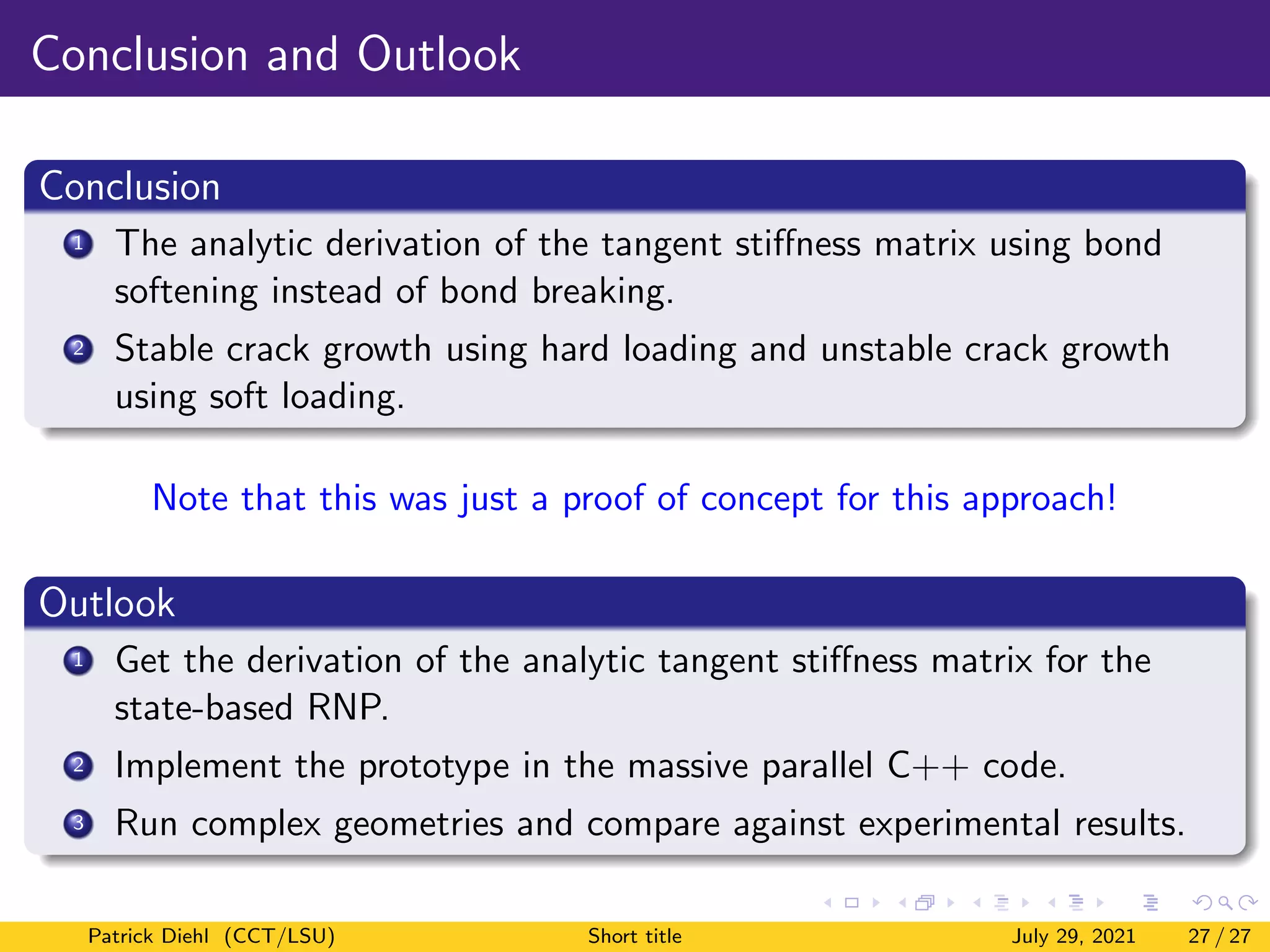
The document discusses a new method for quasistatic fracture simulation using a regularized nonlinear pairwise (RNP) potential. Key points:
1) An analytic tangent stiffness matrix is derived for the RNP potential by taking the derivative of the bond potential, allowing for more efficient simulations.
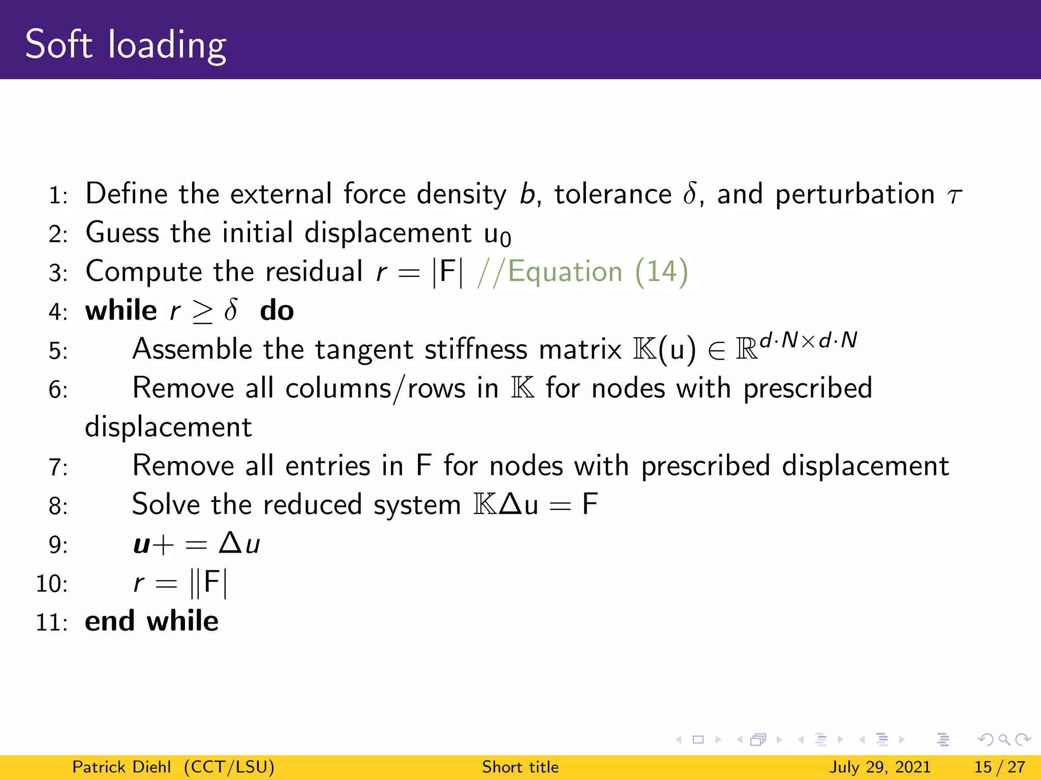
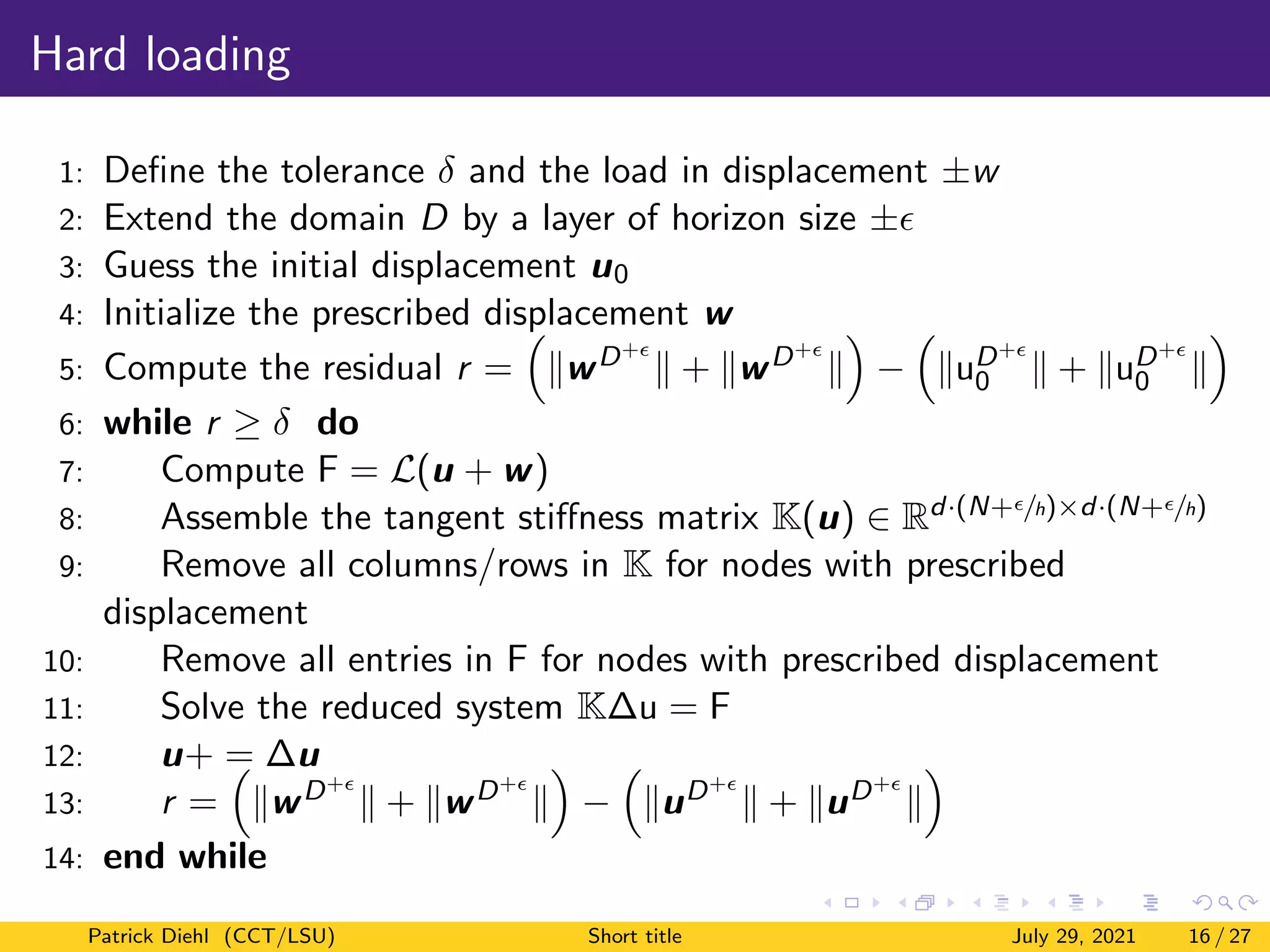
2) Two loading algorithms are presented - soft loading and hard loading. Soft loading uses bond softening while hard loading applies a prescribed displacement field.
3) Numerical results show the method can capture linear elastic behavior, bond softening prior to crack growth, and eventual stable crack propagation under both soft and hard loading conditions.
![Motivation
Observation
Not many quasi-static peridynamic simulations are available due to the
high computational cost in assembling the tangent stiffness matrix using
numerical derivations [1].
Question’s asked
1 Can we use bond softening instead of bond breaking to get some
analytic tangent stiffness matrix?
2 Can we apply hard loading to get stable crack growth?
References
1 Diehl, Patrick, et al. ”A comparative review of peridynamics and phase-field models for engineering fracture
mechanics.” (2021).
Patrick Diehl (CCT/LSU) Short title July 29, 2021 2 / 27](https://image.slidesharecdn.com/lsutemplates-210729210131/75/Quasistatic-Fracture-using-Nonliner-Nonlocal-Elastostatics-with-an-Analytic-Tangent-Stiffness-Matrix-2-2048.jpg)
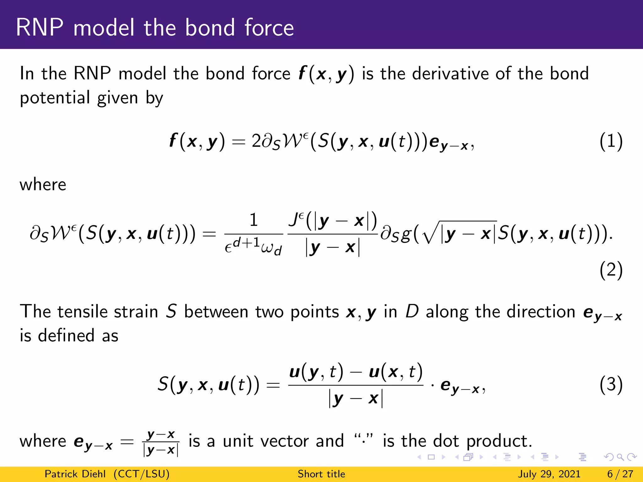
![RNP potential
rc
−rc
r+
−r+
r
g0
(r)
Figure: Cohesive force. The force goes smoothly to zero at ±r+
.
One of the example of g is:
g(r) = C(1 − exp[−βr]) (4)
where C, β are material dependent parameters.
Patrick Diehl (CCT/LSU) Short title July 29, 2021 7 / 27](https://image.slidesharecdn.com/lsutemplates-210729210131/75/Quasistatic-Fracture-using-Nonliner-Nonlocal-Elastostatics-with-an-Analytic-Tangent-Stiffness-Matrix-7-2048.jpg)
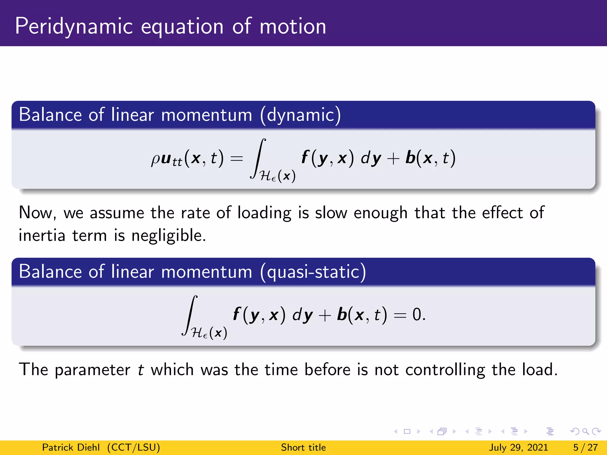
![Quasi-static formulation
For convenience set
L(u)(x) =
Z
H(x)
f (y, x) dy. (5)
We assume at t = 0 that there exists a displacement u0 = u(x, 0) and
body force b(x, 0) for which the displacement is at equilibrium
L(u0)(x) + b(x, 0) = 0, (6)
and the quasistatic evolution u(x, t) : D × [0, T] → Rd is given by
L(u)(x) + b(x, t) = 0. (7)
for a prescribed load path b(x, t) : D × [0, T] → Rd .
Patrick Diehl (CCT/LSU) Short title July 29, 2021 9 / 27](https://image.slidesharecdn.com/lsutemplates-210729210131/75/Quasistatic-Fracture-using-Nonliner-Nonlocal-Elastostatics-with-an-Analytic-Tangent-Stiffness-Matrix-9-2048.jpg)
![Derivation of the tangent stiffness matrix I
We next derive the formula for H(u)[w]. Substituting 1 into 5, and taking
u = u0 + w, we have
L(u0 + w)(x)
=
2
d+1ωd
Z
D∩H(x)
J(|y − x|)
p
|y − x|
g0
(
p
|y − x|S(y, x, u0 + w))ey−x dy,
(8)
From the definition of S in 3, we have
S(y, x; u0 + w) = S(y, x; u0) + S(y, x; w). (9)
Let us do a Taylor expansion for the first derivative of the potential h
g0
(
p
|y − x|S(y, x; u0 + w)) = g0
(
p
|y − x|S(y, x; u0))
+ g00
(
p
|y − x|S(y, x; u0))
p
|y − x|S(y, x; w)
+ O(||w||2
). (10)
Patrick Diehl (CCT/LSU) Short title July 29, 2021 10 / 27](https://image.slidesharecdn.com/lsutemplates-210729210131/75/Quasistatic-Fracture-using-Nonliner-Nonlocal-Elastostatics-with-an-Analytic-Tangent-Stiffness-Matrix-10-2048.jpg)
 =
2
d+1ωd
Z
D∩H(x)
J
(|y − x|)g00
(
p
|y − x|
S(y, x; u0))S(y, x; w)ey−x dy (12)
Note that H(u0)[w] is linear in w.
Patrick Diehl (CCT/LSU) Short title July 29, 2021 11 / 27](https://image.slidesharecdn.com/lsutemplates-210729210131/75/Quasistatic-Fracture-using-Nonliner-Nonlocal-Elastostatics-with-an-Analytic-Tangent-Stiffness-Matrix-11-2048.jpg)